ISSN: 0970-938X (Print) | 0976-1683 (Electronic)
Biomedical Research
An International Journal of Medical Sciences
Research Article - Biomedical Research (2017) Volume 28, Issue 13
Selection of optimum compression algorithms based on the characterization on feasibility for medical image
S. Lalithakumari, R. Pandian*, Jamuna Rani, D. Vinothkumar, Adeline Sneha, Amalarani. V and Bestley Joe
Department of Electronics and Instrumentation Engineering, Sathyabama University, India
- *Corresponding Author:
- R. Pandian
Department of Electronics and Instrumentation Engineering
Sathyabama University, India
Accepted March 07, 2016
Image compression usually comprises of transformation and encoding. Application of different Combinations of these will enable us to find the optimum compression algorithm. In this paper, discrete wavelet transforms and many encoding techniques such as EZW, SPIHT, STW, WDR and ASWDR are used to compress the medical images. In order to evaluate its effectiveness, PSNR and CR are calculated. The optimum compression algorithm is selected based on a compromise between PSNR and CR. The CT images of lung are compressed in this work. To ensure the quality of the proposed algorithm, the feature extraction techniques, which are the pre-request of the classification algorithms, have been found out and the results reveal that the application of compression does not alter the characterization behavior of the medical images.
Keywords
CT Lung image, DWT, Encoder, Image features.
Introduction
Storage and transmission of images require large amount of memory. Image compression techniques overcome this problem by the reduction of storage space and makes sharing of files easier. Image compression applications employ various techniques and algorithms in compressing the images. The techniques can be generally categorized as lossless and lossy compression [1]. Lossy compression technique is used in applications, where a compromise can be made in quality. In lossy compression, there is a minor loss of quality, but the loss is too little to be visible. This technique is preferred in applications where a small amount of compromise on quality of image is accepted. In order to achieve the image compression, the image must be decomposed using suitable transforms [2]. Various transforms are employed for accomplishing this like adaptive lifting, wavelet transform and wavelet packets, etc., Rogerl Claypoole et al. [3] used an Adaptive Lifting scheme for image reduction and obtained a PSNR of 38.5d b for Doppler, Blocks etc. Rogerl Claypoole et al. [4] applied Wavelet lifting methodology for image reduction for a cameraman image and it was measured with a PSNR of 42db. Cadder bank et al. [5] implemented Wavelet Transforms based image reduction for different images such as Bike, Café, Water and X-rays. In their work, entropy was employed as a figure of merit and it was found as 5.90. Minh N. Do et al. [6] used in Contourlet Transforms for both peppers and Barbara images. In their work also, entropy was evaluated as 30.47 db. Gemma Piella et al. [7] applied wavelet lifting scheme for various images such as Rectangular, Crosses, Houses and Peppers. The performance is found with the entropy values. Chenwei Deng [8] applied DWT-Seam carving Methodology for a test image and bit – rate was used a figure of merit and it was found as 0.09. In this work, discrete wavelet transform is used for transforming the image and is primarily used for decomposition of images, where as encoding is used to achieve the entire compression process and Embedded Zero Tree wavelet is adopted to achieve the image compression. In this research, a CT normal lung and cancer affected lung image with axial view are used for compression process. After the compression process, the quality of the image is evaluated by the values of PSNR. The amount of compression is estimated with the value of Compression ratio, which is the ratio of the sizes of original and compressed sizes of images. The paper is formulated in the following way. Chapter 2 elucidates the transform technique and Chapter 3 describes the encoding techniques. Feature extraction methodology is expressed in chapter 4. Results and discussion is enumerated in chapter 5 and this proposed work is concluded in Chapter 6.
Wavelet Transforms
In wavelet analysis, images are represented by a set of basic functions. A single prototype function called the mother wavelet is used for deriving the basis function, by translating and dilating the mother wavelet. The wavelet transform can be viewed as a decomposition of an image in the time scale plane. In this work symlet with vanishing moment 2 used. The basic and compact wavelet, which is proposed by Daubechies is an orthonormal wavelets, which is called as Daubechies wavelet. It is designed with extremely phase and highest number of vanishing moments for a given support width. Associated scaling filters are minimum-phase filter. Daubechies wavelets are generally used for solving fractal problems, signal discontinuities, etc. The symlets are nearly symmetrical wavelet, which are also proposed by Daubechies as modifications to the db family. Daubechies proposed modifications of her wavelets that increase their symmetry can be increased while retaining great simplicity. The symlets have properties similar to daubechies [9].
Encoding
Encoding is performed in compression, for the reduction of the redundant data and elimination of the irrelevant data. In this work, Embedded zero tree wavelet (EZW), Set Partitioning In Hierarchical Trees (SPIHT), Spatial-orientation Tree Wavelet (STW), Wavelet Difference Reduction (WDR) and Adaptively Scanned Wavelet Difference Reduction (ASWDR) are used.
Embedded zero tree wavelet
The embedded zero tree wavelet algorithm (EZW) is an image compression algorithm, in which embedded code represents a sequence of binary decisions which distinguishes an image from the “null” image EZW which leads the compression results [10].
Spatial-Orientation tree wavelet
STW is basically the SPIHT algorithm; the only difference is that SPIHT is slightly more cautious in its organization of coding output. The only difference between STW and EZW is that STW uses a different approach to encoding the zero tree information. STW uses a state transition model. The locations of transformed values undergo state transitions, from one threshold to the next [11].
Set partitioning in hierarchical trees
This algorithm applies a spatial orientation tree structure, which can be able to extract significant coefficients in wavelet domain. SPIHT does not have flexible features of bit stream but, it supports multi-rate, and it has high signal-to-noise ratio (SNR) and good image restoration quality, hence, it is suitable for a high real-time requirement [12].
Wavelet difference reduction
The term difference reduction is used to represent the way in which WDR encodes the locations of significant wavelet transform values, Although WDR will not produce a higher PSNR The significance pass is the difference between WDR and the bit-plane encoding [13,14].
Feature extraction
Since, the accuracy of a classification system mainly based on the proper choice of the features, it is necessary to identify a good set of features. In this proposed work, a gray-level co-occurrence matrix (GLCM) is employed, which is a statistical method that utilizes the spatial relationship of pixels. Davis et al. [15] initiated the application of gray level co-occurrence matrix (GLCM) in order to find out the features that are to be generated based on a pixel’s neighborhood. Davis t al. [15] continued the work of in such a way of the directional distribution of GLCM features and proposed a set of polarogram statistics which are rotationally invariant. Haralick et al. [16] suggested that rotation invariant features could be obtained from co-occurrence matrices by taking the average and range of each feature type over the four angles that is used. The gray-level difference statistics is another texture description method, which is closely related to GLCM, Weszka et al. [17]. A co-occurrence matrix, also referred to as co occurrence distribution, is defined over an image to be the distribution of co-occurring values at a given offset. Represents the distance and angular spatial relationship over an image sub-region of specific size. The GLCM is created from a gray-scale image. The GLCM calculates how often a pixel with gray-level (grayscale intensity or Tone) value i occurs either horizontally, vertically, or diagonally to adjacent pixels with the value j. A well-known statistical tool for extracting second-order texture information from images is the grey-level co-occurrence. The GLCM matrix is one of the most popular and effective sources of features in texture analysis. For a region, defined by a user specified window, GLCM is the matrix of those measurements over all grey level pairs. In this method, features are calculated based on the absolute differences between pairs of gray-levels or average gray levels instead of original gray-level pixel values. This approach makes the statistics a little more robust to illumination variations than in the case of GLCM. The gray level co occurrence matrix is extracted from the above mentioned images. The features, extracted from the CT Lung images are tabulated in Tables 3 and 4.
| Algorithm | PSNR | CR |
|---|---|---|
| ezw 1 | 60.03 | 74.44 |
| ezw 3 | 52.15 | 44.08 |
| ezw 5 | 42.22 | 17.52 |
| ezw 7 | 33.24 | 5.87 |
| ezw 9 | 28.528 | 2.66 |
| SPIHT 1 | 41.61 | 90.95 |
| SPIHT 3 | 42.86 | 21.95 |
| SPIHT 5 | 35.9 | 7.37 |
| SPIHT 7 | 31.81 | 4.03 |
| SPIHT 9 | 27.91 | 1.85 |
| STW 1 | 60.27 | 67.25 |
| STW 3 | 47.06 | 29.38 |
| STW 5 | 37.56 | 10.12 |
| STW 7 | 32.91 | 5.5 |
| STW 9 | 28.59 | 2.44 |
| wdr 1 | 40.34 | 71.92 |
| wdr 3 | 40.94 | 50.22 |
| wdr 5 | 41.01 | 19.86 |
| wdr 7 | 32.75 | 6.5 |
| wdr 9 | 28.54 | 2.83 |
| ASWDR 1 | 40.39 | 70.13 |
| ASWDR 3 | 40.94 | 48.56 |
| ASWDR 5 | 41.01 | 19.45 |
| ASWDR 7 | 32.75 | 6.51 |
| ASWDR 9 | 28.54 | 2.83 |
Table 1. Normal CT Lung _axial view using Symlet 2 with Encoding Methods for various decomposition level.
| Algorithm | PSNR | CR |
|---|---|---|
| ezw 1 | 60.3 | 77.27 |
| ezw 3 | 52.2 | 44.36 |
| ezw 5 | 41.82 | 16.55 |
| ezw 7 | 33.6 | 5.54 |
| ezw 9 | 29.13 | 2.55 |
| SPIHT 1 | 46.5 | 87.83 |
| SPIHT 3 | 43.54 | 21.95 |
| SPIHT 5 | 35.96 | 6.8 |
| SPIHT 7 | 32.14 | 3.72 |
| SPIHT 9 | 28.23 | 1.78 |
| STW 1 | 60.32 | 65.51 |
| STW 3 | 46.92 | 29.64 |
| STW 5 | 37.48 | 9.59 |
| STW 7 | 33.48 | 5.27 |
| STW 9 | 28.9 | 2.43 |
| wdr 1 | 46.5 | 71.05 |
| wdr 3 | 47.4 | 50.6 |
| wdr 5 | 40.79 | 18.96 |
| wdr 7 | 33.09 | 6.24 |
| wdr 9 | 28.84 | 2.78 |
| ASWDR 1 | 46.5 | 69.57 |
| ASWDR 3 | 47.4 | 48.81 |
| ASWDR 5 | 40.79 | 18.4 |
| ASWDR 7 | 31.94 | 6.16 |
| ASWDR 9 | 28.84 | 2.75 |
Table 2. Cancer affected CT Lung _axial view using Symlet 2 with Encoding Methods for various decomposition level.
| Features | Uncompressed image | Compressed image with high PSNR (60.03 dB) | Compressed image with LowPSNR (27.91 dB) |
|---|---|---|---|
| Image Entropy | 5.73 | 5.74 | 6.65 |
| Auto correlation | 21.56 | 21.44 | 21.42 |
| Contrast | 0.56 | 0.56 | 0.32 |
| Correlation | 0.92 | 0.92 | 0.95 |
| Cluster prominence | 535.46 | 528.28 | 480.05 |
| Cluster shade | 82.96 | 82.17 | 69.05 |
| Dissimilarity | 0.25 | 0.25 | 0.21 |
| Sum of square | 21.71 | 21.59 | 21.45 |
| Sum of average | 8.52 | 8.49 | 8.52 |
| Sum of variance | 61.93 | 61.53 | 59.51 |
| Sum of entropy | 1.61 | 1.61 | 1.73 |
| Difference variance | 0.56 | 0.56 | 0.33 |
| Difference entropy | 0.59 | 0.59 | 0.55 |
| Information measure of correlation 1 | 0.61 | 0.61 | 0.64 |
| Information measure of correlation | 0.89 | 0.89 | 0.91 |
| INN | 0.97 | 0.97 | 0.98 |
| Energy | 0.31 | 0.31 | 0.29 |
| Maximum probability | 0.52 | 0.51 | 0.49 |
| Sum of variance | 21.71 | 21.59 | 21.45 |
| Sum of average | 8.52 | 8.52 | 8.51 |
| Entropy | 1.82 | 1.82 | 1.95 |
| Homogeneity | 0.91 | 0.91 | 0.91 |
| Inverse measure | 0.89 | 0.89 | 0.91 |
| IDN | 0.97 | 0.97 | 0.98 |
Table 3. Features of CT Normal Lung- axial view image.
| Features | Uncompressed image | Compressed image with high PSNR (60.3 dB) | Compressed image with Low PSNR (28.23dB) |
|---|---|---|---|
| Image Entropy | 5.84 | 5.85 | 6.69 |
| Auto correlation | 23.87 | 23.71 | 23.83 |
| Contrast | 0.57 | 0.56 | 0.38 |
| Correlation | 0.95 | 0.95 | 0.96 |
| Cluster prominence | 834.2 | 829.56 | 805.34 |
| Cluster shade | 114.76 | 114.38 | 103.55 |
| Dissimilarity | 0.26 | 0.25 | 0.22 |
| Sum of square | 24.01 | 23.86 | 23.89 |
| Sum of average | 8.59 | 8.56 | 8.59 |
| Sum of variance | 65.98 | 65.78 | 64.55 |
| Sum of entropy | 1.98 | 1.95 | 2.06 |
| Difference variance | 0.57 | 0.56 | 0.39 |
| Difference entropy | 0.61 | 0.59 | 0.56 |
| Information measure of correlation 1 | 0.65 | 0.66 | 0.67 |
| Information measure of correlation | 0.94 | 0.94 | 0.95 |
| INN | 0.97 | 0.97 | 0.97 |
| Energy | 0.19 | 0.2 | 0.18 |
| Maximum probability | 0.36 | 0.37 | 0.35 |
| Sum of variance | 24.01 | 23.86 | 23.89 |
| Sum of average | 8.59 | 8.56 | 8.59 |
| Entropy | 2.23 | 2.21 | 2.3 |
| Homogeneity | 0.91 | 0.91 | 0.91 |
| Inverse measure | 0.94 | 0.94 | 0.95 |
| IDN | 0.97 | 0.97 | 0.98 |
Table 4. Features of CT Cancer affected Lung- axial view image.
Results and Discussion
In this work, CT image of lung is undergone the proposed algorithms. Discrete wavelet transform based decomposition was performed on the image. Symlet2 is used for decomposing the image. After the decomposition, five encoding methods are adopted. The ability of the compression algorithms are evaluated in terms of PSNR and CR. This is tabulated in Tables 1 and 2.
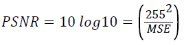
The PSNR between two images having 8 bits per pixel in terms of decibels (dBs) is given by:
Compression ratio = No. of bits in original image/ No. of bits in compressed image
Generally when PSNR is 40 dB or greater, then the original and the reconstructed images are virtually indistinguishable by human eyes. The compression ratio of the image is given by No. of bits in original image/ No. of bits in compressed image. PSNR and CR values of the different encoding methods are expressed in Tables 1 and 2. The original and compressed images of normal Lung (axial view) and Cancer affected Lung images are shown in Figures 1a-1c and 2a-2c, respectively.

Figure1. a Low CR (90.15%) b.High CR (68.72%) c. Uncompressed Normal Lung _sagittal view image(Jpeg).

Figure 2. a High PSNR (60.03 dB) b. Low PSNR(40.39 dB) c. Uncompressed Normal Lung _axial view image(Jpeg).
References
- Sachin D. A review of image compression and comparison of its algorithms. IJECT 2011; 2: 22-26.
- Said A, Pearlson WA. An image multi resolution representation for lossless and lossy compression, IEEE transaction 1996; 9: 1303-1310.
- Claypoole R, Nowak RD. Adaptive wavelet transforms via lifting. IEEE International conference on image processing 1998; 3: 1513-1516
- Claypoole R, Davis G, Sweldens W, Baraniuk R. Non linear Wavelet transform for image coding via lifting. IEEE Transaction on image processing 2003; 12: 1449-1459.
- Cadderbank AR. Loss less image compression using integer to integer wavelet transforms. International Conference on image processing 1997; 1: 596-599.
- Do MN. Countourlet transform: An efficient directional multi resolutional image representation. IEEE Transaction on image processing 2005; 14: 2091-2106
- paella G. Adaptive lifting schemes combiming semi norms for lossless image compression. IEEE International conference on image processing 2005; 1: 753-756
- Deng C, Lin W, Cai J. Content-Based Image Compression for Arbitrary-Resolution Display Devices. IEEE Transactions on Multimedia 2012; 4: 1127-1139.
- Hong-wei MA, Bin W. Application of Wavelet Transform to Signal de-noising in Ultrasonic Testing. NDT 2004; 26: 68-71.
- Wei Z. Advanced Technology of Wavelet Analysis Based on MATLAB. Published by XiDian University Press,Xi’an; 8: 203-208.
- Kim BJ, Xiong Z, Pearlman Wa. Low bit Rate, Scalable Video coding with 3D Set Partitioning in Hierarchical Trees. IEEE Transactions on circuits and system for video technology 2000; 10.
- Tian J, Wells RO. A lossy image codec based index coding. IEEE Data Compression Conference DCC 1996; 456.
- Tian, J, Wells RO. Image data processing in the compressed wavelet domain, 3rd International Conference on Signal Processing Proc. Yuan, B.and Tang. Beijing, China 1996; X. Eds. 978–981.
- Shapiro JM. Embedded image coding using zerotrees of wavelet coefficients.IEEE Transactions on Signal Processing. 41: 3445-3462.
- Davis L, Johns S, Aggarwal J. Texture analysis using generalized co-occurrence matrices. IEEE Transactions on Pattern Analysis and Machine Intelligence. PAMI 1979; 1: 251-259.
- Haralick RM, Shaunmugam K, Dinstein I. Textural features for image classification. IEEE Transactions on Systems, Man and Cybernetics SMC 1973; 3: 610-621.
- Weszka JS, Dyer CR, Rosenfeld A. A Comparative Study of Texture Measures for Terrain Classification in Systems, Man and Cybernetics. IEEE Transactions on SMC 1976; 6: 269-285.