ISSN: 0970-938X (Print) | 0976-1683 (Electronic)
Biomedical Research
An International Journal of Medical Sciences
Research Article - Biomedical Research (2018) Volume 29, Issue 8
Risks reduction control techniques analysis in type-1 diabetes
Hajra Arif, Sana Shuja, Shehryar Imtiaz, Ali Khaqan*, Qadeer ul Hasan, Shahzad A. Malik, Junaid Ahmed and Raja Ali Riaz
COMSATS Institute of Information Technology, Islamabad, Pakistan
Accepted date: February 5, 2018
DOI: 10.4066/biomedicalresearch.29-17-3740
Visit for more related articles at Biomedical ResearchType 1 diabetes mellitus is one of the most common childhood diseases which, if not carefully mitigated, can pose menacing risks like hyperglycemia and ketoacidosis, ultimately leading to heart disease, kidney failure and other life-threatening complications. In order to reduce these risks, two existing control schemes are implemented with the purpose of simulation-based comparative analysis between linear and nonlinear control strategies. In this regards, H1 is selected as a nonlinear strategy whereas lead-lag compensation is the choice from the class of classical linear strategies. The designed control scheme consists of three main components: a controller, an Insulin Feedback Loop (IFL) and a Safety Mechanism (SM). IFL is designed such that it modifies the loop gain for the reduction of postprandial hypoglycemia risks, and the SM predicts the future glucose levels and acts accordingly by modifying the controller output to reduce the risk of hypoglycemia and hyperglycemia. The comparison of the transient and dynamic performances in terms of rise time, settling time and overshoot of both controllers is analysed. It is observed that the H1 gives a far sturdy response as compared to the lead-lag controller.
Keywords
Lead-lag, Hyperglycemia, Hypoglycemia, H1, Type 1 diabetes
Introduction
Diabetes mellitus type 1 is a type of diabetes in which insulin deficiency is observed due to an autoimmune destruction of the pancreatic-cells, ultimately resulting in high blood sugar levels. This disease, being one of the most common unpreventable maladies, requires self-management through regular insulin injections and continuous monitoring of blood glucose. The latter needs intense care and therefore, is extremely demanding. To avoid the states of hyperglycemia and hypoglycemia, a T1DM patient must constantly observe the blood glucose level throughout his life, which ultimately leads to ineffective glycemic control. The exact number of people affected globally is unknown, although it is estimated that about 80,000 children develop the disease each year [1]. Therefore, automatically controlling the blood glucose level in TIDM patients is a long-standing problem [2-8].
Diabetes is growing at a rate of 3-4 % per year in youths [9], with children being the mainly affected group [10]. Due to this fact, considerable clinical and bioengineering advancement has been made in this field. In this regards, artificial pancreas is a technology introduced for diabetic patients to automatically control their blood glucose level by the pro-vision of the substitute endocrine functionality of a healthy pancreas. It contains a Continuous Insulin Infusion (CSII) pump, a continuous blood glucose monitoring (CGM), and a control algorithm. Strategies like Model Predictive Control (MPC), Proportional Integral Derivative (PID) and adaptive control have been broadly implemented both in silico and in clinical trials [11-17]. Moreover, other control techniques like H1 control [18-20] and Linear Parameter-Varying (LPV) control [21] have also been considered, though but both these techniques have not yet been tested in silico.
Due to the uncertainty and time-varying properties of a system, great difficulty is faced when dealing with long actuation delays or the large inter as well as intra-patient discrepancy, which creates a need of some tuning to every individual patients’ characteristics for achieving high-closed loop performance [22]. This can be done by using certain a priori clinical information which is easily accessible e.g., the patient’s Total Daily Insulin (TDI). Although, due to the complex and time consuming nature of this process it is likely to become almost impracticable to implement, nonetheless, a general model is presented considering each patients’ TDI.
In this study, a comparative analysis is conducted between two well-known linear and nonlinear controllers and their design procedure is presented (H1 and lead-lag) on a third-order model, whose gain is personalized by subjects’ TDI. The comparison is done between the transient parameters like rise time, settling time and overshoot. For avoiding the state of hypoglycemia, the addition of Insulin Feedback Loop (IFL) has been made, which appropriately regulates an estimate of patient’s Insulin on Board (IOB) by controlling the insulin infusion when excessive plasma insulin concentration is appraised. Furthermore, for reducing the risks of hypoglycemia and hyperglycemia, an SM is added which modifies the controller output. It consists of two prediction strategies followed by a decision algorithm which jointly enhance the chances of better prediction (over a 20 min horizon) of dangerous future glucose scenarios, hence achieving a more robust system.
This paper is organized as follows. The model identification is performed in section II. Sketching of root locus and controller designs are shown in section III. Results of comparative analysis are displayed in section IV and conclusions are presented in section V.
System Model and Patient Tuning
Research on T1DM has resulted in various models that describe the insulin-glucose dynamics [23,24]. For control synthesis, a simple lower-order model is more desirable than a complex, sophisticated model [25]. Moreover, to avoid the high level of difficulty faced in maintaining accurate amount of glucose in closed loop system caused by patient-model mismatch or physiological significance of model parameters, a lower-order control-relevant model is chosen, using black-box approach and adjustments are made based entirely on a priori patient data.
For each in-silico adult of the distribution version of the T1DM simulator, a linear model of the transfer characteristics from the insulin delivery (pmol/min/kg) to the deviation from a particular glucose concentration (mg/dl) is identified. Three glucose concentrations are considered here: 90, 120 and 150 mg/dl in order to capture the frequency response at different operating points. Hence, three linear models are obtained for each patient. The model used for simulation is defined in detail in [26]. The procedure of identification process is briefly explained below.
First, the basal insulin that produces the particular glucose concentration at steady state is obtained which is then added to a sinusoidal insulin sweep. This signal is introduced through a CSII pump, over a period of 12 h and a sampling time of Ts=10 min [26]. This process resulted in third-order models for all 30 cases by using a sub-space identification algorithm [27]. In view of these models, the following third-order discrete time transfer function is defined.
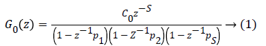
Where C0 =0.132, p1=0.965, p2=0.95, p3=0.93. The values are chosen such that the gain is overestimated and the phase is kept lower than all other identified models in order to obtain robustness. Figure 1 shows the bode diagram of G0 (z). A controller based on this nominal model could be too conservative, therefore, in order to limit this conservatism, an individualized transfer function G0,j (z) is defined as,

Figure 1: Bode diagram of G0 (z).
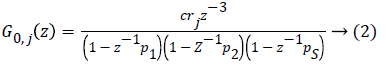
Here, rj is based on 1800 rule, the factor which is divided into 1800 is the total daily insulin of each individual patient. This parameter represents the gain, which changes according to the individual patient’s TDI where the TDI of the patient with index j is denoted by TDIj, hence Tj=1800/TDIJ and

is a scaling constant. This limits the conservatism by the adaptation of crj to each individual patient instead of the constant value c0.
Control Techniques and Design
The scheme comprises of three parts: a controller, a SM and an IFL. A schematic diagram of the closed loop system is depicted in Figure 2. In which r and e are the reference and error signals, respectively. KSM,j is the controller, modified by which is the output of SM, g is glucose concentration, usm is the output of the controller, and u is the insulin input that is commanded to the CSII pump. Finally, is a switching signal which predicts the glucose values. If low glucose values are predicted by the SM, then the controller suspends or attenuates the glucose delivery and if high glucose level is predicted then the insulin delivered by the controller is increased. This paper only focuses on the design of the controllers and comparison of the results and more information on the model can be found in [26].

Figure 2: Block diagram of the control scheme.
The controllers are designed such that they have a small steady state tracking error to follow the reference signal which is based on the response of an average normal patient to a 100 g glucose disturbance at t=0. This response can be represented as the impulse response of a second order system defined as,
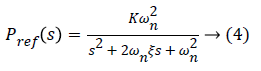
Where (ωn)=0.02 and damping ratio (ξ)=0.7. The continuoustime transfer function of Equation 2 can be written as,
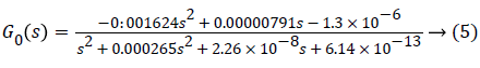
A. Pole-zero gain analysis
1) Determining the root loci on real axis: The design process of the lead-lag controller is performed by applying the principle of root locus. The first step in sketching the root locus plot is to locate the open-loop poles and zeros in the complex s-plane. From Equation 2 we get 3 poles at s=0:0593 × 10-3 (p1), s=0:0858 × 10-3 (p2), and s=0.1201 × 10⁻³ (p3) and 2 zeros at s=0.0024+0.0014i (z1) and s=0.0024 0:0014i (z2) (one zero is at infinity) as shown in Figure 3. Where a pole is indicated by a cross and a zero by circle. The root locus branches starts from open loop poles and end at finite or infinite zeros. It exists on real axis to the left of an odd number of poles and zeros. Here, the number of individual root loci is three as it has three open-loop poles. The root locus exists from the p2 to z2, p1 to z1 and p3 to +1.

Figure 3: Pole-zero map of G0(s).
2) Determine the asymptotes of the root loci: Asymptotes are defined as number of finite poles (n) of G (s) H (s)-number of finite zeros (m) of G (s) H (s).
q=n-m → (6)
Where, q=1. Furthermore, the angles of asymptotes are given by,
where k=0 represents the asymptotes with the smallest angle with the real axis (σ). For q=1 and k=0, yields ± 180. All the asymptotes intersect with real axis at a centroid (α) given by,
Where Σn pi=-1.0354 × 10⁻³, Σmzi=4.86 × 10⁻³, which yields α= -5:89 × 10-3. However, this point is not on root locus as the sum of angles in question to this point from open-loop poles and zeros of the system, is not equal to 180 so centroid does not exist on locus.
3) Find the break-away and break-in points: Break-away or break-in points occur when N (s) D’ (s) N' (s) D(s)=0, where N (s) is the numerator polynomial and D (s) is the denominator polynomial of the plant, and (’) represents the derivative of the respective polynomial. Here,
N (s) D’ (s)-N’ (s) D (s)=0:001624s4+1.5809 × 10⁻⁵s3-3.6867 × 10⁻⁸s2-6.9102 × 10⁻¹²s-2.9867 × 10⁻¹⁶.
gives 4 roots at s=0.0053, 0.0046, -0.00011, -7.1e-005. Not all of these roots are on the locus. From these 4 real roots, 3 roots at s=0.0053, 0.0046, -0.00011 exist on the locus. So the root locus shall start from these three points and end on the openloop finite or infinite zeros of the system.
4) Determine the angle of departure/arrival: For accurate sketching of root loci, one must find the directions of roots. Since there are no complex poles so there is no angle of departure however, there are two complex zeros in the loop gain so angle of arrival exists and is defined as 180-(sum of angles of vectors to a complex zero with respect to other zeros) +(sum of angles of vectors to a complex zero with respect to poles). Determining the angles each open-loop pole zero makes with the complex zero z1=0.00243+0.00144j
θz=(-0.00243+0.00144j)-(-0.00243+0.00144j)
θz=+jº
p1=((-0.00243+0.00144j)-(0.0593 × 10⁻³))
p1=(-2.37010 3+0.00144j)=-31.28º
p2=((-0.00243+0.00144j)-(0.0858 × 10⁻³))
p2=(-2.344 × 10⁻³+0.00144j)=-31.56º
p3=((-0.00243+0.00144j)-(1.207 × 10⁻⁴))
p3=(-2.309 × 10⁻³+0.00144j)=-31.94º
Angle of arrival is equal to:
θarrival=180º-θz+p1+p2+p3
θarrival=180º-90º+(-31.28º-31.56º-31.94º)
θarrival=-4.78º=-175.22º
From the above calculations the root locus can be plotted as shown in Figure 4, where each branch is shown in a different color.

Figure 4: Root locus of G0(s).
The open-loop step response of the transfer function mentioned in Equation 2 is depicted in Figure 5 which is showing the rise time, settling time and peak response. It is clear from the step response that the needed specifications are not met and the response is not approaching the required final value so a controller must be designed to generate the desired results. Mentioned below are the two low-order, practical controllers designed to reduce the risks of hyper and hypoglycemia.

Figure 5: Open-loop step response of G0(s).
B. H∞ controller
H∞ techniques are synthesized to minimize the closed loop impact of a disturbance, the impact either being measured in terms of stabilization or performance. It also offers high disturbance rejection and high stability [28]. The design procedure starts by representing the system according to the standard configuration as depicted in Figure 6 [29].

Figure 6: Standard configuration for designing H8 controller.
Here, the input w is combination of the reference signal and disturbances and u is the manipulated variables. The matrices G and K represent the plant and the controller, respectively. There are two outputs, z is the error signal that should be minimized and y is the variable used to control the system. A controller is designed such that it keeps a check on the tracking error and effectively measures the strength of control action. This method is used to attain the optimal solution in terms of the lowest gain between the input disturbance and the output errors and is known as mixed sensitivity problem.
A discrete H∞ controller Kj is synthesized, considering Adult j with G0,j (z) being its nominal model, solving a mixedsensitivity problem with a performance objective defined in [26] as:
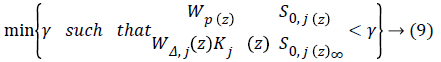
Here, S0,j (z)=(1+G0,j (z) Kj) (z))-1 is defined as the sensitivity function, Wp (z) is performance weight and WΔ,j (z) is control weight. The sample-period is 10 min.
Wp (z) and WΔ,j (z) are:
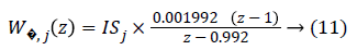
where ISj is the individualized gain based on the subject’s sensitivity to insulin and is defined in [26]. Step response after applying the mixed-sensitivity problem is shown in Figure 7, after conversion to continuous state.

Figure 7: Closed-loop step response of Kj.
C. Lead-lag compensator
A lead-lag compensator is one of the fundamental building blocks in classical control theory. It is used to control the undesired frequency response by the placement of poles and zeros such that the transient response changes correspondingly. Both lead and lag compensators add a pole-zero pair into the open loop transfer function. In the lead controller the zeros are placed closer to origin than the poles whereas in lag controller the poles are placed closer to origin than the zeros in the left half plane. The pole-zero pair is placed near to the origin and the distance between them is kept minimum so that it does not affect the transient parameters and only deal with steady-state error. Lead compensator is used to improve the system transient response by providing phase lead at higher frequencies which moves the root locus further in the left half plane, thereby improving stability, while lag compensator is used to reduce steady state error by providing phase lag at low frequencies. Both the compensators can be represented by,
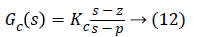
where |p|>|z| for a lead controller, and |p|<|z| for a lag controller.
A lead-lag compensator is made by cascading a lead and a lag compensator. It gives the benefits of both lead and lag compensator by improving stability and reducing steady state error simultaneously. It is represented by
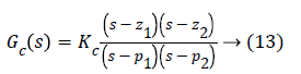
Where, z1 and p1 represent the zero and pole of lead compensator, whereas z2 and p2 represent the zero and pole of lag compensator. The exact location of poles and zeros of the compensator to be designed are determined by the specification like natural frequency and damping ratio through which settling time and overshoot can be found and then the controller can be designed accordingly. Design of controller is presented below.
1) Determine desired location for dominant closed-loop poles: As it is depicted in the figure below, the desired closedloop poles (represented by boxes) location is the point where the lines of wn and intersect, which is -0.0141+0.0142i.
It is clear from Figure 8 that simple loop gain adjustments will Figure 9. Angles used to determine the deficient angle not yield desired results so a lead controller must be inserted to meet the design requirements.

Figure 8: Desired pole location indicated by intersection of the lines representing wn and ξ.

Figure 9: Angles used to determine the deficient angle ф
2) Find the deficient angle: In order for a point to exist on root locus, sum of angles of all the poles (p)-sum of angles of all the zeros (z) must be equal to 180º, otherwise a controller should be so designed that poles and zeros of the controller contribute to the angle deficiency and dominant closed-loop poles acquire the desired location on the new root locus.
The angle from the pole p1 to the desired dominant closed-loop pole at s=-0.0141+0.0142i is 134.4º (α). Angle from p2 to s=134.6º (γ) and angle from p3 to s=-134.4º (β) as shown in Figure 9.
θp= αº+γº+βº= 403.4º → (15)
Now calculating θz, angle from z1 to the desired dominant closed-loop pole location (s) is 142.2 (δ1) and angle from z2 to s is 136.7º (δ2) which gives:
θz=(δ1)+(δ2)=278.7º → (16)
By using Equation 14, we see that the equation is not satisfied, hence we now know that this point does not exists on root locus so now we find the deficient angle As depicted in Figure 9.
ф=180º-p+z → (17)
Using Equation 17, ф can be calculated as:
ф=180º-403.4º+278.9º=55.1º → (18)
In the present system, the angle G (s) at the desired dominant closed-loop pole can be calculated as:
G (s)s=-0.0141+0.142j=124.5º → (19)
For the desired point s s-0.0141+0.142j to exist on root locus a controller should be designed such that its poles and zeros give a total angle of 55.1º so that Equation 20 is satisfied.
124.5º+p-z=180º → (20)
3) Designing the controller: In the first step, the gain is set to a negative value since the root locus extends to positive infinity which ultimately leads to the system becoming unstable as the poles tend to go to zeros and in this system one zero is at infinity. Then, placing, arbitrarily, the first pole at -0.02605 making an angle of 49.9º and zero at 0.0001867 making an angle of 134.29º with the desired dominant closed-loop pole. The total angle from this pole-zero pair sums up to 84.39º which creates a need of 2nd pole-zero pair. Placing the 2nd pole at -0.038529 making an angle of 30.17º and zero at 0:00017311 making an angle of 134.4º with the desired dominant closedloop pole, respectively. Adding the angle generated by previous pole-zero pair with this pole-zero pair generates a total angle of 188.62º. Now, placing a 3rd pole-zero pair such that it satisfies Equation 20 so that the dominant closed-loop poles acquire the desired location. By placing the pole at -0.057706 and zero at -0.00023611, Equation 20 is satisfied as they make a total angle of 116.28º.
θp=49.9º+30.17º +18.03º=98.1º → (21)
z=134.29º+134.4º+134.31º=403º → (22)
which satisfies Equation 20 as:
124.5º+98.1º-403º ≈ 180º → (23)
By the addition of three lead compensators the dominant closed-loop poles now reside on the desired position on the root locus as shown in Figure 10 represented by pink boxes lying on the intersection of the lines of wn and ξ, but the steady state error is still present as depicted in Figure 11.

Figure 10: Root locus of controller Gc(s).

Figure 11: Closed-loop step response of Gc(s) showing steady-state error.
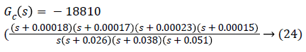
To reduce this steady state error, a lag compensator shall be added such that it does not change the shape of the root locus. The angle contribution from this pole-zero pair should be minimum so that the transient parameters do not change but only the steady state error reduces [30,31]. By placing, arbitrarily, the pole at 0 (origin) and zero at -0.00015264, we get the desired result with no change in the shape of root locus. The final result is shown in Figure 12. By plotting the above scenario, following 4th-order transfer function with gain k=-18810 is generated.

Figure 12: Closed-loop step response of Gc(s).
In classical control theory, different compensators are used to achieve the desired result. In this scenario, lead-lag compensator proved to be the best as it gave minimum damping and overshoot while keeping the order low, which makes the system stable and hence increases the chances of its implementation in real life.
A Comparative Analysis
Two different control schemes are employed in order to reduce the risks of hyperglycemia and hypoglycemia in type 1 diabetes mellitus. H∞ controller gave better results due to its non-linear nature which ensures stabilization with guaranteed performance. Moreover, it is readily applicable to problems involving multivariate systems. On the other hand, lead-lag controller gave poor performance due to the restrictions offered by its linear nature. However, amongst the classical control strategies, lead-lag compensator proved to be the optimal choice for this scenario as it gives same pole placement as H∞. Furthermore, the complexity caused due to the H∞ is also reduced.
Table 1 compares the different time domain specifications of both the controllers. Here, it can be clearly seen that the values of rise time and settling time of H∞ controller are much lesser than that of lead-lag controller while keeping the gain higher. It can also be seen that both systems give no overshoot whereas H∞ controller shows a considerable amount of oscillations, Out (1) taking 9774 s to settle down to the steady-state value and Out (2) taking 11739 s to get to the steady-state value. Keeping these results in mind, H∞ controller gives better performance hence leading to a more robust system.
| Controller | Gain | Rise time (s) | Settling time (s) |
|---|---|---|---|
| H∞ | 3900 | ||
| to Out (1) | 826 | 1.06 × 10⁴ | |
| to Out (2) | 61.2 | 1.18 × 10⁴ | |
| Lead-lag | -18810 | 1.33 × 10⁵ | 2.31 × 10⁵ |
Table 1. Comparison of non-linear and linear controllers.
This scheme is practical because it uses a priori data which leads to more reliable results. The SM assists the algorithm in preventing low glucose outcomes by prediction of future glucose values, The IFL reduces the risks of postprandial hypoglycemia and finally H∞ controller which gave better performance, than lead-lag compensator, helps maintain the glucose value by delivering the right amount of insulin.
Conclusion
A simulation-based comparative analysis is conducted for the purpose of risks reduction in type 1 diabetes. The robust H∞ controller is designed via a mixed-sensitivity problem and a lead-lag controller is designed such that both controllers maintain the glucose level near to the reference value. The transient parameters are compared to see which controller performs better. The h∞ controller showed good performance and minimal hyper- and hypoglycemia risks as compared to the lead-lag controller.
Conflict of Interest
The authors have no conflict of interest regarding the publication of this manuscript.
References
- Chiang JL, Kirkman, MS, Laffel LMB, Peters AL. Type 1 diabetes through the life span: a position statement of the American Diabetes Association. Diab Care 2014.
- Cobelli C, Dalla-Man C, Sparacino G, Magni L, De Nicolao G, and Kovatchev BP. Diabetes: models, signals, and control. IEEE Rev Biomed Eng 2009; 2: 5496.
- Wilinska M, Hovorka R. Simulation models for in silico testing of closed-loop glucose controllers in type 1 diabetes. Drug Discovery Today Dis Models 2008; 5: 289298.
- Bonda J, Veh J, Palerm C, Herrero P. El pancreas artificial: Control automatico de infusi on de insulina en. Diabetes Mellitus tipo I Revista Iberoamericana de Automatica e Inform atica Industrial 2010; 7: 520.
- Cobelli C, Renard E, Kovatchev B. Artificial pancreas: past, present, future. Diabetes J 2011; 60: 2672-2682.
- Atlas E, Thorne A, Lu K, Phillip M, Dassau E. Closing the loop. Diab Technol Therap 2014; 16: 23-33.
- Bequette BW. Challenges and progress in the development of a closed loop artificial pancreas. Proc Am Control Conf Montreal Canada 2012; 4065-4071.
- Doyle FJ, Huyett LM, Lee JB, Zisser HC, Dassau E. Closed-loop artificial pancreas systems: engineering the algorithms. Diab Care 2014; 37: 11911197.
- Kaufman FR. Medical management of type 1 diabetes. Alexandria VA USA: Am Diab Assoc 2012.
- Escher S, Li Afrese T, Sandholzer H. The epidemiology of type 1 diabetes mellitus. Type 1 Diab 2013; 122.
- Steil G, Darwin K, Hariri F, Saad M. Feasibility of automating insulin delivery for the treatment of type 1 diabetes. Diabetes 2006; 55: 3344-3350.
- Grosman B, Dassau E, Zisser HC, Jovanovic L, Doyle FJ. Zone model predictive control: A strategy to minimize hyper-and hypoglycemic events. J Diabetes Sci Technol 2010; 4: 961975.
- Breton M, Farret A, Bruttomesso D, Anderson S, Magni L, Patek S, Dalla-Man C, Place J, Demartini S, Favero SD, Toffanin C, Hughes Karvetski C, Dassau E, Zisser H, Doyle FJ, De Nicolao G, Avogaro A, Cobelli C, Renard E, Kovatchev B, The International Artificial Pancreas Study Group. Fully integrated artificial pancreas in type 1 diabetes: Modular closed-loop glucose control maintains near normoglycemia. Diabetes 2012; 61: 2230-2237.
- Cobelli C, Dalla-Man C, Sparacino G, Magni L, De Nicolao G, Kovatchev BP. Multinational study of subcutaneous model-predictive closed-loop control in type 1 diabetes mellitus: summary of the results. J Diab Sci Technol 2010; 4: 1374-1381.
- Hughes CS, Patek SD, Breton M, Kovatchev BP. Anticipating the next meal using meal behavioral profiles: a hybrid model-based stochastic predictive control algorithm for T1DM. Comp Met Prog Biomed 2011; 102138-148.
- Zarkogianni K, Vazeou A, Mougiakakou SG, Prountzou A, Nikita KS. An insulin infusion advisory system based on autotuning nonlinear model-predictive control. IEEE Trans Biomed Eng 2011; 58: 2467-2477.
- Wilinska M, Chassin L, Acerini C, Allen J, Dunger D, Hovorka R. Simulation environment to evaluate closed-loop insulin delivery systems in type 1 diabetes. J Diab Sci Technol 2010; 4: 132-144.
- Colmegna P, Sanchez Pena R. Analysis of three T1DM simulation models for evaluating robust closed-loop controllers. Comp Met Prog Biomed 2014; 113: 371-382.
- Ruiz-Velazquez E, Femat R, Campos-Delgado D. Blood glucose control for type I diabetes mellitus: A robust tracking H1 problem. Control Eng Pract 2004; 12: 1179-1195.
- Parker RS, Doyle FJ, Ward JH, Peppas NA. Ro-bust H1 glucose control in diabetes using a physiological model. J AICHE 2000; 46: 2537-2549.
- Sanchez Pena RS, Ghersin AS, Bianchi FD. Time-varying procedures for insulin-dependent diabetes mellitus control. J Electr Comput Eng 2011; 2011: 10.
- Patek SD, Bequette BW, Breton M, Buckingham BA, Dassau E, Doyle FJ, Lum J, Magni L, Zisser H. In silico preclinical trials: methodology and engineering guide to closed-loop control in type 1 diabetes mellitus. J Diab Sci Technol 2009; 3: 269-282.
- Sorensen JT. A physiologic model of glucose metabolism in man and its use to design and asses improved insulin therapies for diabetes. Ph.D. Dissertation Massachusetts Inst Technol Cambridge MA USA 1985.
- Dalla MC, Robert AR, Claudio C. Meal simulation model of the glucose-insulin system. IEEE Trans Biomed Eng 2007; 54: 1740-1749.
- Snchez Pea R, Bianchi F. Model selection: from LTI to switched LPV. Proc Am Control Conf Montreal Canada 2012; 156-166.
- Colmegna P. Reducing risks in type 1 diabetes using h1 control. IEEE Trans Biomed Eng 2014; 61: 2939-2947.
- Overschee PV, de Moor B. Subspace algorithms for the identification of combined deterministic and stochastic systems. Automatica1994; 30: 7593.
- Bansal A, Veena S. Design and analysis of robust H-infinity controller. Control Theory Inform 2013; 3: 7-14.
- Hu Z, Salcudean SE, Loewen PD. Robust controller design for teleoperation systems. Sys Man Cybern 1995.
- Beale G. Compensator design to improve steady-state error using root locus. Classical Systems Control Theory 2001.
- Teixeira MCM. Direct expressions for Ogatas lead-lag design method using root locus. IEEE Trans Educ 1994; 37: 63-64.