ISSN: 0970-938X (Print) | 0976-1683 (Electronic)
Biomedical Research
An International Journal of Medical Sciences
Research Article - Biomedical Research (2017) Health Science and Bio Convergence Technology: Edition-II
Intima-media thickness segmentation using weighted graph based active contour technique
Ashokkumar L1* and Rajendran P2
1Department of Computer Science and Engineering, K. S. Rangasamy College of Technology, Tiruchengode, Tamil Nadu, India
2Department of Computer Science and Engineering, Knowledge Institute of Technology, Salem, Tamil Nadu, India
- *Corresponding Author:
- Ashokkumar L
Department of Computer Science and Engineering
K. S. Rangasamy College of Technology
Tiruchengode, India
Accepted on November 15, 2016
Segmentation of ultrasound images is a challenging task due to the lower contrast and the speckle noise. Active contour is one of the most widely used techniques for ultrasound image segmentation. This method has drawbacks such as the predefined initial curve position and the number of contour points to be considered. A new active contour segmentation for extracting the intima media layer and plaque in the Common Carotid Artery (CCA) ultrasound images is presented in this paper. This paper has proposed a fuzzy weighted graph based active contour segmentation technique to overcome all these drawbacks. The proposed method is used for segmenting Intima-Media Thickness (IMT) and plaque in common carotid artery B-mode ultrasound images to assess the risk of stroke in the human subject under investigation. Using canny edge detection and connected component analysis methods, the initial contour was determined and applied as input to the proposed active contour segmentation algorithm. The proposed algorithm was compared with five conventional methods. Experimental results prove that the proposed approach has produced better results than traditional methods. The overall probability of error achieved by the proposed algorithm was 5.28%, which was very less compared to other conventional methods.
Keywords
Intima-media thickness, Plaque, B-mode ultrasound images, Active contour, Fuzzy weighted graph
Introduction
In recent years, stroke is one of the most important causes of death in the world. It is the foremost cause of long term disability. IMT and plaque are used as an important indicator for the risk prediction. This paper is aimed to provide the modified graph based active contour segmentation method for identifying the risks of stroke. The proposed algorithm performs the lumen, intima, and media layers and plaque segmentation for CCA images.
For biomedical applications, segmentation task is usually not simple. Snakes provide a powerful interactive tool for image segmentation [1]. The convergence of snake contours depends on the interaction of internal and external forces, where the minimum energy can be found. The internal force is based on the assumption that the contour is continuous and smooth, while the external force is used to extract the desired characteristics, such as edges. Critical issues of deformable contour methods include complex procedures, multiple parameter selection, and sensitive initial contour location. To represent the unknown interfaces, the level set method is the most elegant due to its ability in dealing with unknown topology. The curve is represented by a level set formulation, and the energy minimization problem is solved by a level set evolution. A drawback of the level set method is expensive computation. To solve these problems, edge based contour detection and graph based segmentation are more efficient [2].
Hongzhi et al. presented an approach to image segmentation that prefers edges rather than segment boundaries [3]. Segmentation was performed based on the intensity distribution distinct from that of the surrounding background. A measure called Minimal Description Length framework was used to measure the figure’s distinctiveness. An edge and region information was combined to overcome the local ambiguities of edge detection. It can be extended it to open contours as long as the contour can be considered as organizing the image into distinct regions. Krit et al. introduced a new edge following technique for boundary detection in noisy images [4]. This method can detect the boundaries of objects using the information from the intensity gradient via the vector image model and the texture gradient via the edge map. It was compared with the Active Contour Models (ACM), geodesic active contour models, active contours without edges, gradient vector flow snake models, and ACMs based on vector field convolution. This method was robust and applicable on various kinds of noisy images without prior knowledge of noise properties.
Bahadir et al. proposed a simulated annealing-based optimal threshold detection method in edge-based segmentation of grayscale images [5]. Simulated Annealing (SA) was used to obtain an optimal segmentation result, which is better and more preferable than the classical methods, namely, Otsu’s method (for bi-level segmentation) and Snake method (for edge-based segmentation). Optimal threshold has been obtained for bilevel segmentation of grayscale images using entropy-based simulated annealing method. This threshold was used in determining optimal contour for edge-based image segmentation of grayscale images. When probability differences between white class (foreground) and black class (background) were minimized, threshold value was maximized. An optimal contour detection was obtained using pixel coordinates of contour control points as distances of p-median locations.
Graph-based segmentation aims to merge spatially neighbouring pixels which are of similar intensities into a Minimal Spanning Tree (MST), which corresponds to a sub graph (i.e. a sub region). The image can be grouped into several sub regions (i.e. a forest of MST). A graph-based method of active contour models called network snakes was investigated. This method enables a free optimization of arbitrary graphs representing the geometric position of networks and boundaries between adjacent objects. The main impacts of network snakes were the combination of the image energy representing objects in the real world, the internal energy incorporating shape characteristics, and the topology representing the structure of the scene. The new method of active contour models was represented by a graph to incorporate the topological characteristics of a contour network. The topology of the contour within the graph was defined by the nodes, which were characterized by the degree of nodes. Nodes with a degree were represented as end points of a contour. Nodes with a degree of 2 represent a normal part of a contour and nodes with a degree greater than 2 represent nodes in which more than two edges terminate.
An interactive image segmentation method based on Multiple Piecewise Constant with Geodesic Active Contour (MPC-GAC) model was proposed [6]. The MPC model can segment objects and background more accurately than Chan and Vese model. This model has achieved better boundary capturing properties. The new MPC-GAC energy functional can be iteratively minimized by graph cut algorithms with high computational efficiency compared with the level set framework. This iterative algorithm alternates between the piecewise constant functional learning and the foreground and background updating so that the energy value gradually decreases to the minimum of the energy functional. The k-means method was used to compute the piecewise constant values of the foreground and background of image. A graph cut method was used to detect and update the foreground and background. Using graph cut optimization, the MPC-GAC model can effectively segment images with inhomogeneous objects and background.
This paper presents a new model for active contours to detect objects in an image, based on techniques of graph evolution. The proposed model can detect objects whose boundaries are based on the edge gradient, texture gradient and energy. These measures are used as weights for evolving the active contour, which will stop on the desired object boundary. In this paper, we propose a fuzzy weighted graph-based active contour technique to locate the lumen-intima and media-adventitial interfaces on common carotid artery ultrasound images for IMT segmentation. Experiments demonstrate that the proposed model is better and more robust than classical snake methods.
Methods
Common carotid artery
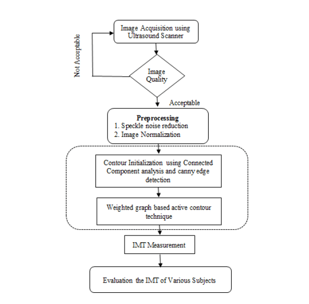
Ultrasound B-mode scanning is used for visualizing near wall and far wall of CCA. Intima, Media and Adventitia are the three different layers of CCA wall. Figure 1 shows the anatomy of common carotid artery. IMT refers to the distance between intima-lumen interface and media-adventitia interface. It is used as a validate measurement for risks of CCA [7].

Figure 1. Anatomy of common carotid artery.
Proposed segmentation algorithm
The proposed methodology for B-mode CCA images consist of the General Processing, Pre-processing, Finding Analysis and test the various subjects. It shown in Figure 1.
Pre-processing
Speckle noise is considered as a major performance limiting factor for ultrasound image analysis. It has reduced both image contrast and detail resolution. There is always a trade-off between noise suppression and loss of information. De-speckling is an important pre-processing step in ultrasound image segmentation. It keeps as much of important information as possible. It helps to improve the performance of segmentation techniques that is followed in the later section. Bilateral filter has been proved to be an efficient and effective method for speckle reduction. Histogram Equalization is then applied for image contrast adjustment. This equalization technique is very effective for image that has low contrast.
Contour initialization
Templates can be extracted using edge detection methods. There are many ways to perform edge detection [8]. However, the majority of different methods may be grouped into two categories, gradient and Laplacian. The gradient method detects the edges by looking for the maximum and minimum in the first derivative of the image. The Laplacian method searches for zero crossings in the second derivative of the image to find edges. Canny edge detection works best when compared to the various edge detection algorithms. It uses a gradient approach. This is done by the following steps.
1) Applying noise smoothing to the original image.
2) Filtering the original image using a set of eight kernels.
3) Estimating the local edge gradient magnitude at each pixel.
4) Produce the output as the maximum response of all 8 kernels at each pixel location.
The Canny edge detection consists of a set of eight 3 × 3 convolution kernels. It estimates the approximate image gradient of each pixel by convolving the image with a set of eight 3 × 3 kernels. The kernels can be applied separately to the input image, to produce the gradient component in each direction. Each of the kernels is sensitive to an edge orientation ranging from 0° to 315° in steps of 45°, where 0° corresponds to a vertical edge. For each pixel, the value of the corresponding pixel in the output magnitude image is the maximum response |G| obtained using Equation 8. The values for the output orientation image lie between 1 and 8, depending on which of the 8 kernels produced the maximum response.
An approximate magnitude is represented as |G| and calculated by the following
|G| = max (|Gi|), i=1….n
Where Gi is the response of the kernel i at the particular pixel position and n is the number of convolution kernels. The edge magnitude and orientation of a pixel is then determined by the template that matches the local area of the pixel the best.
Connected component analysis scans an edge detected image and group its pixels into components based on pixel connectivity. Different measures of connectivity between pixels are available. All the pixels in the component should share similar pixel intensities. After groups are determined, each pixel can be assigned with a gray level or color according to the group it belongs to.
Consider two pixels p and q. A pixel p at (x, y) has four direct neighbours, N4 (p) and four diagonal neighbours, ND (p). Eight neighbours of a pixel, NS (p) can be defined as the union of N4 (p) and ND (p). Possible connectivity between pixels p and q are: 1) 4 connectivity if q is in N4 (p), 2) 8-connectivity if q is in NS (p), and 3) m-connectivity if q is in N4 (p), or if q is in ND (p) and N4 (p) N4 (q)=ϕ
In the proposed algorithm, 8-pixel connectivity is used. It scans the image produced by the template matching method. Scanning is done along a row until it reaches a pixel p for which the value is 1. Connectivity checks are carried out by checking the labels of pixels that are North-East, North, North- West and West of the current pixel, which is shown in Figure 2.

Figure 2. 8-Neighborhood mask.
Assume that array A is used to represent the image. It consists of M rows and N columns. A [x, y] refers to the element in column x and row y, with x ε {0, N-1}, y ε {0, M-1}. Let B be an array that has the same size as A. This array can be used to hold the connected component labels. Let L represents the label index. Start with L=0 and increment L whenever a new connected component label is created. The goal is to end up with all of the pixels in each connected component having the same label and all of the distinct connected components having different labels.
There is a possibility that some of the pixels in the same connected component will end up with different labels. These conflicts can be resolved at the end of the labelling process using equivalences between neighbouring labels.
Algorithm
Input: Binary image
Output: Connected components (each region has unique label)
Method:
First pass: Identifying the connected components
1. Scan each pixel in the image from top to bottom, left to right.
2. If the current pixel element is not the background
a) Check the northeast, north, northwest, and west pixel for a given region.
b) If none of the neighbours match with the intensity of the current pixel, then assign new region value to the current pixel.
c) If only one neighbor matches, then assign pixel to that region value.
d) If multiple neighbours match and are all members of the same region, assign pixel to their region.
e) If multiple neighbours match and are members of different regions, assign pixel to one of the regions.
f) Store the equivalence between neighbouring labels.
Second pass: Resolving label conflicts
1. Scan each pixel in the image from top to bottom, left to right.
2. If the element is not the background then
Re-label the element with the lowest equivalent label.
The output of the connected component analysis technique is used as initial contour for proposed graph based active contour algorithm.
Fuzzy weighted graph based active contour
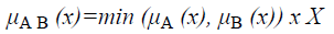
To extract the region of interest, these detected edges were used as templates for the proposed fuzzy based graph algorithm. Graphs are a very important model of networks. The weights of the arcs are not always crisp but fuzzy [9]. A graph is an ordered pair (V, E) which consists of two sets V and E, where V is the set of vertices or nodes, and Eis the set of edges or links). Graphs may be of two types: undirected graphs and directed graphs. In an undirected graph, the edge (i, j) and the edge (j, i) are identical unlike that in the case of directed graph.
In this paper, we consider fuzzy weighted undirected graphs [10], vertices and edges remain crisp, but the edge weights will be fuzzy numbers. A fuzzy quantity is defined as a fuzzy set in the real line R, that is, an R → [0,1] mapping A. If A is upper semi-continuous, convex, normal, and has bounded support, then it is called a fuzzy number. If X is a universe of discourse, a fuzzy set A in X is a set of ordered triplets A={x, A (x) : x X}, where (x): X → [0, 1] are functions such that 0 ≤ (x) ≤ 1 for all x X. For each x X, the value (x) represent the degree of membership of the element x to A X.
A graph was constructed from the given image into a Minimal Spanning Tree (MST), which corresponds to a sub graph (i.e. a sub region of the image). The image can therefore be grouped into several sub regions (i.e. a forest of MST). Obviously, the step for emergence of pixels into a MST is the key, determining the final segmentation results. A pairwise region comparison was also performed to determine whether or not a boundary between two sub graphs should be eliminated.
Algorithm
Step 1: Set the initial contour using edge templates for extracting the region of interest.
Step 2: Construct a graph G for each region in an image. In G, each pixel corresponds to a vertex and an edge connects two vertices based on weights. The edge weight is defined as fuzzy weight based on edge and texture gradients and energy features.
Step 3: Sort the edges in E in non-descending order in terms of the edge weight.
Step 4: Select the ith edge in the sorted edges. If the ith edge is a valid edge (i.e. it connects two different subgraphs) and the boundary between the two subgraphs can be eliminated with respect to the pairwise region comparison, the two subgraphs are merged into a larger subgraph and this edge is set to be invalid.
Step 5: Repeat Step 4 until all edges in E have been traversed.
When all edges have been traversed, a forest including a number of MSTs can be obtained. Each MST corresponds to a sub region in the image.
Fuzzy sets
A fuzzy set [9] is completely determined by its membership function. The set of support of a fuzzy set A is the set of all elements x of X for which (x, μA (x)) A and μA (x)>0 holds. A fuzzy set A with the finite set of support {a1, a2, a3…an} can be described in the following way
Where 
The membership function for the union of two sets A and B can be defined as
and corresponds to the maximum of the corresponding coordinates in the geometric visualization. The membership function for the intersection of two sets A and B is given by
Definition 1: Let A and B be fuzzy sets of the universe of discourse U with the membership functions μA and μB respectively. Then, A is a subset of B, denoted as A B, if and only if
μA (u) μB (u) for all u U
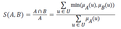
Definition 2: Let A and B be fuzzy sets of the universe of discourse U, and let μA and μB be the membership functions of the fuzzy sets A and B, respectively. The fuzzy subset hood S (A, B) measures the degree, in which A is a subset of B,
Let A be a fuzzy set of the universe of discourse U, where U={u1, u2, u3…un}, A= μA (u1) | u1+ μ2 (u2)+…..+μA (un)/un,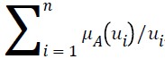 , and let α be a real value between zero and one. The α-level-cut Aα-level of the fuzzy set A is defined as follows:
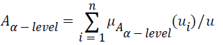
Where if μA (ui) ≥ α, then let μAα-level (u1); if μA (ui)<α, then let μAα-level (ui)=0
Parameters computation
During graph construction, the next vertex was selected based on the comparison of the edge gradient magnitude, texture gradient and energy features for its neighbourhood. Each component is the convolution between the image and the corresponding difference mask.
At the position (i, j) of an image, the successive positions of the edges are then calculated by a 3 × 3 matrix
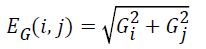
N (I, j)=αEG (i, j)+βD (I, j)+γTG (i, j)+εE (i, j), 0 ≤ i ≤ 2, 0 ≤ j ≤ 2
where α, β, γ and ε are the weight parameters that control the edge to flow around an object. The larger value of N (i, j) indicates the stronger edge in the corresponding direction.
The 3 × 3 matrices EG (i, j), D (i, j), TG (i, j) and E (i, j) are calculated as follows:
The image gradient EG (i, j) of each pixel is calculated by convolving the image with a pair of 3 × 3 filters. These filters estimate the gradients in the horizontal (i) and vertical (j) directions. The magnitude of the gradient is calculated using:
and gradient direction can be calculated using:
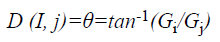
where EG (i, j) and D (i, j) are the average magnitude and direction of edge, represents the texture gradient obtained from Laws texture masks, and E (i, j) represents the energy function. The value of each element in the above three matrices are ranged between 0 and 1.
The texture gradient TG (i, j) are computed by convolving an input image with each of the Law’s texture masks. The 2D mask used for texture discrimination is generated by L × LT.
The Gi mask highlights the edges in the horizontal direction while the Gi mask highlights the edges in vertical direction. After taking the magnitude of both, the resulting output detects edges in both directions.
If n represents the number of points on the contour, the distance between every point is equal to 360/n. Each point in the contour has to be evaluated based on energy minimization principle. The energy function E (i, j) is defined by the following
Where E denotes the total energy of the contour, Ein denotes the internal energy, and Eex denotes the external energy. After summing up the values for each point in the contour, choose the contour with minimum energy as the best one. When the value of energy function does not change, contour deformation stops and segmentation process ends at that point. If x and y are the coordinates of the image I (x, y), contour is defined using S (p)=(x (p), y (p), p [0, 1]. The internal energy and external energy are computed using the following

Where α (p) represents the contour’s bending ability and β (p) represents the contour strength.
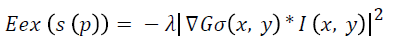
Where λ denotes the external weight factor and Gσ (x, y) is the 2D Gaussian function with standard deviation σ.
Weights optimization
Simulated Annealing (SA) algorithms are usually better than greedy algorithms, when it comes to problems that have numerous locally optimum solutions. It guarantees a convergence upon running sufficiently large number of iterations.
A general SA algorithm starts with a randomly chosen initial solution. A neighbor solution is generated by the required changes for computed objective function and appropriate mechanism [11]. This mechanism is a random search. It practices both the decreasing alterations and increasing alterations of the value of objective function. The possibility of getting a worse solution at initial temperature and higher temperatures is quite high. A better or worse solution is obtained depending on the cooling schedule and the temperature of the system. The move from existing solution to a new neighbor solution is done depending on the energy comparison. The simulated annealing algorithm performs the following steps:
1. The algorithm generates a random trial point. The algorithm chooses the distance of the trial point from the current point by a probability distribution with a scale depending on the current temperature.
2. The algorithm determines whether the new point is better or worse than the current point. If the new point is better than the current point, it becomes the next point. If the new point is worse than the current point, the algorithm can still make it the next point. The algorithm accepts a worse point based on an acceptance function. The probability of acceptance is
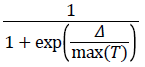
where
Δ=new objective-old objective.
T0=initial temperature
T=current temperature.
Since both Δ and T are positive, the probability of acceptance is between 0 and 1/2. Smaller temperature leads to smaller acceptance probability. Also, larger Δ leads to smaller acceptance probability.
3. The algorithm systematically lowers the temperature, storing the best point found so far.
4. The algorithm stops when the average change in the objective function is small or when it reaches any other stopping criterion.
Algorithm Pseudocode SIMULATED-ANNEALING
Begin
temp=INIT-TEMP;
solution=INIT-SOLUTION;
while (temp>FINAL-TEMP) do
new_solution= neighbor (solution);
ΔC=COST (new_solution) –COST (solution);
if (ΔC<0) then
solution=new_ solution;
else if (RANDOM (0,1)>e-(ΔC/temp)) then
solution=new_ solution;
temp=Decrease (temp);
End
Initially the solution is obtained with values 0.1 for α, β, γ and ε parameters. New solution is then generated with different parameter values. If the difference between the new solution and the old solution is less than zero, then new solutions is considered as old solution and repeat the procedure by lowering the temperature value. Otherwise, solution is accepted based on the probability function.
Experimental Results
Philips HD11XE US Machine with high resolution Aloka Prosound Alpha-10 ultrasound scanner and compact linear array transducer is used for the data acquisition of the images. A multi-frequency linear transducer is operated at the frequency range 7-10 MHz for recording arterial movements. The transducer is placed exactly at the starting point of the bifurcation of CCA to obtain lumen for different subjects. Video recorder is used for recording movements for a period of 10 s for each subject. Recorded video shows the transverse and longitudinal section of CCA. It is converted into frames and then stored as still images for further analysis. Still images can be used to measure the IMT of CCA.
In GED and EF algorithms, the result of the traditional edge detection method was considered as the initial contour. For SAOT, the initial contour was determined using entropy based simulated annealing method. These initial contours were closer to true object boundaries. For graph based segmentation methods such as NS and MPC-GAC, initial contours were determined manually [12,13]. The proposed algorithm combines the benefits of the above two categories of algorithms. The proposed algorithm determines the initial contour using canny edge detection method. To obtain the final optimal contour, weight parameters such as α, β, γ and ε are adjusted between 0 and 1. The result of the proposed method was selected from the best experimental results of the parameter settings. The performance of the proposed method was tested by comparing its results with the results from classical contour models. Figure 3 shows the results of different edge detection methods. The performance of three conventional edge based contour detection methods such as Generalized Edge Detection (GED), Edge Following (EF), and Simulated Annealing based.

Figure 3. Result of edge detection methods. (a) Original image, (b) Sobel, (c) Prewitt, (d) Roberts, (e) Laplacian of Gaussian, (f) Zero crossing, (g) Canny.
Optimal Threshold (SAOT) and two graph based detection methods such as Network Snakes (NS) and Multiple-Piecewise Constant Geodesic Active Contour MPC-GAC) were shown in Figures 4-8. Conventional methods did not perform well in IMT and plaque segmentation. Compared to conventional boundary detection methods, Fuzzy Weighted Graph based Active Contour algorithm was proposed to achieve good segmentation results which were shown in Figure 9. The results of detecting the object boundaries in noisy images show that the proposed technique is much better than the five contour models. Speckle noise is the most challenging issue in Ultrasound segmentation. To remove this noise, bilateral filter is used in this research work. Histogram equalization technique is used to enhance the quality of an image.

Figure 4. Generalized edge detection. (a) Original image, (b) Segmented image.

Figure 5. Edge following. (a) Original image, (b) Segmented image.

Figure 6. Simulated annealing based optimal threshold detection. (a) Original image, (b) Segmented image.

Figure 7. Network snakes. (a) Original image, (b) Segmented image.

Figure 8. MPC-GAC segmentation. (a) Original image, (b) Segmented image.

Figure 9. Proposed segmentation. (a) Original image, (b) Segmented image.
To evaluate the efficiency of the proposed method, Probability of Error (PE) is computed as follows

where P (O) and P (B) are priori probabilities of objects and background in images. P (B|O) is the probability of error in classifying objects as background and vice versa. The average PEs of the conventional methods such as GED, EF, SAOT, NS, MPC-GAC models, and the proposed method are 11.53%, 10.88%, 8.09%, 7.21%, 7.76%, and 5.28%, respectively.
A total of 177 subjects under different ages and sex were considered for experimenting the proposed method. Table 1 shows the intima media thickness of normal subjects in different age groups. IMT values were greater for male than female IMT mean and SD values for male in the range of 0.48 mm to 0.79 mm and ± 0.01-± 0.05 mm respectively. IMT mean and SD values for females in the range of 0.43 mm- 0.78 mm and ± 0.02-± 0.04 mm respectively. Table 2 shows IMT of abnormal subjects under different age groups. From this table, it was inferred that most of the people under the age group of 30-60 were suffered from pathologies such as Hypertension and Atherosclerosis [14].
| S. No | Age Groups in year | Sex | Number of subjects | Intima-media thickness IMTmean ± SD (mm) |
|---|---|---|---|---|
| 1 | 21-30 | Male | 17 | 0.48 ± 0.05 |
| Female | 10 | 0.43 ± 0.04 | ||
| 2 | 31-40 | Male | 9 | 0.61 ± 0.02 |
| Female | 12 | 0.58 ± 0.02 | ||
| 3 | 41-50 | Male | 22 | 0.66 ± 0.01 |
| Female | 16 | 0.65 ± 0.02 | ||
| 4 | 51-60 | Male | 8 | 0.74 ± 0.01 |
| Female | 7 | 0.74 ± 0.01 | ||
| 5 | 61-70 | Male | 24 | 0.79 ± 0.01 |
| Female | 20 | 0.78 ± 0.02 |
Table 1. Intima-media thickness of normal subjects.
| S. No | Age Groups in year | Number of subjects | Intima-media thickness IMTmean ± SD (mm) | Name of pathology |
|---|---|---|---|---|
| 1 | 30-60 | 25 | 1.45 ± 0.05 | Hypertension |
| 2 | 30-60 | 7 | 2.35 ± 0.42 | Atherosclerosis |
Table 2. Intima media thickness of abnormal subjects.
Conclusion
A new edge based technique was designed for weighted graph based boundary detection and applied it to object segmentation problem in medical images. This technique includes feature information such as edge gradient, edge direction, texture gradient and energy. The proposed technique was applied to detect the object boundaries in several types of noisy images where the ill-defined edges were encountered. The performance of the proposed algorithm was evaluated using PE and execution time [15]. It was better by comparing the results of five existing methods such as GED, EF, SAOT, NS and MPC-GAC shown in Figures 10-12. The observed results indicate that the segmented images reveal the rate of prediction of Intima Media Thickness in the cardiovascular and cerebrovascular pathologies [16].

Figure 10. Comparative analysis.

Figure 11. Probability error rate for different algorithms.

Figure 12. Execution time for various algorithms.
References
- Kass M, Witkin A, Terzopoulos D. Snakes: active contour models. Int J Comput Vision 1988; 1: 321-331.
- Felzenswalb P, Huttenlocher D. Efficient graph-based image segmentation. Int J Comp Vis 2004; 59: 167-181.
- Hongzhi W, John O. Generalizing edge detection to contour detection for image segmentation. Comp Visi Imag Unders 2010; 114: 731-744.
- Krit S, Nipon TU, Sansanee A. Boundary detection in medical images using edge following algorithm based on intensity gradient and texture gradient features. IEEE Trans Biomed Eng 2011; 58.
- Bahadir K, Serdar K. A simulated annealing-based optimal threshold determining method in edge-based segmentation of grayscale images. Appl Soft Comp 2011; 11: 2246-2259.
- Wenbing T, Xue-Cheng T. Multiple piecewise constant with geodesic active contours (MPC-GAC) framework for interactive image segmentation using graph cut optimization. Image Vis Comput 2011; 29: 499-508.
- Santhiyakumari N, Rajendran P, Madheswaran M. Medical decision-making system of ultrasound carotid artery intima-media thickness using neural networks. J Dig Imag 2011; 24: 1112-1125.
- Shin MC, Goldgof D, Bowyer KW. Comparison of edge detector performance through use in an object recognition task. Comp Vis Image Unders 2001; 84: 160-178.
- Zadeh LA. Is there a need for fuzzy logic. Inform Sci 2008; 178: 2751-2779.
- Chris C, Peter DK, Etienne EK. Shortest paths in fuzzy weighted graphs. Int J Intel Sys 2004; 19: 1051-1068.
- Dimitris B, John T. Simulated annealing. Stat Sci 1993; 8: 10-15.
- Gerardo MRE, Mariano R, Ioannis AK. Segmentation of the luminal border in intravascular ultrasound B-mode images using a probabilistic approach. Med Image Anal 2013; 17: 649-670.
- Ilea DE, Duffy C, Kavanagh L, Stanton A, Whelan PF. Fully automated segmentation and tracking of the intima media thickness in ultrasound video sequences of the common carotid artery. Ultras Ferroelectr Freq Contr IEEE Trans 2013; 60.
- Sakthivel K, Jayanthiladevi A, Kavitha C. Automatic detection of lung cancer nodules by employing intelligent fuzzy c-means and support vector machine. Biomed Res 2016; S123-S127.
- Lumia R, Shapiro L, Zuniga O. A new connected components algorithm for virtual computers. Comp Vis Graph Image Proc 1983; 22: 287-300.
- Iana S. Intima-media thickness: Appropriate evaluation and proper measurement, described. E J Cardiol Pract 2015; 13.