ISSN: 0970-938X (Print) | 0976-1683 (Electronic)
Biomedical Research
An International Journal of Medical Sciences
Research Article - Biomedical Research (2016) Computational Life Sciences and Smarter Technological Advancement
Discrete Tchebichef moment based machine learning method for the classification of disorder with ultrasound kidney images
1Department of Electronics and Communication Engineering, Sree Sowdambika College of Engineering, Tamil Nadu, India
2Department of Electrical and Communication Engineering, Mepco Schlenk Engineering College, Sivakasi, Tamil Nadu, India
- *Corresponding Author:
- S Bama
Department of Electrical and Communication Engineering
Sree Sowdambika College of Engineering
India
Accepted on August 12, 2016
Medical imaging provides a mean to visualize internal organs of human body, their anatomy as well as their functionality. Out of the many imaging modality such as CT, MRI, PET etc, ultrasound imaging of soft tissues is the safest one. However, the low contrast images of ultrasound modality poses the classification task as challenging one. A novel and effective approach for the classification of abnormalities in ultrasound B mode kidney images using Discrete Tchebichef Moment (DTM) is proposed. Instead of considering the whole kidney regions for the abnormality classification, typical blocks from the parenchyma (i.e cortex, medulla) and central sinus regions of kidney have been considered. Tchebichef kernels that are unique and not the rotational representation of existing kernels are carefully selected to extract the features from each of these blocks. A multiclass Support Vector machine (SVM) classifier with 5 fold cross validation has been used to carry out the classification. Performance of the proposed work is analysed with a dataset comprising of 160 samples from 40 images, Hu’s invariant features and Grey Level Co-occurance Matrix (GLCM) features are also extracted and fed as input to the multiclass SVM for comparative analysis. Quantitative evaluation metrics such as accuracy, precision, recall and fscore have been computed to reveal the performance of the proposed method. Promising results produced by the proposed work reveals the scope of Computer Aided classification of disorders in ultrasonic kidney images.
Keywords
Computer aided diagnosis, Ultrasound imaging, Discrete tchebicheff moment, Multi class SVM.
Introduction
Ultrasound imaging modality is a prevalent imaging tool in assessing the internal organs of human. The non-invasive, nonradiation, low cost as well as less patient preparedness characteristics of this modality makes ultrasound imaging a superior one compared to other imaging modalities such as MRI, CT and PET. Also, this is the most preferred modality for the children and pregnant women and is found useful in diagnosing the soft tissues like kidney, liver, uterus etc [1]. Presence of speckle noise, low contrast image and inherent artefacts of this modality makes the interpretation by the radiologists as a subjective one. Even experts may have interobserver variation as well as intra-observer variation in some situations. A possible objective aid in decision making to assist the radiologists can be a significant contribution by the engineering research community to this modality.
In a broader sense, a computer assisted Diagnosis (CAD) system can be useful in assisting the doctors in circumferences such as early detection of diseases, quantifying the level of severity, distinguishing one abnormality from a closely related another abnormality etc. A successful CAD system depends upon the image acquisition protocol, image processing algorithms at various stages and the allowed level of interaction of expert with the CAD [2,3]. By enhancing salient features and suppressing the background noise, a CAD can assist doctors in improving the qualitative analysis. Analysing the features of an image quantitatively can be made useful in delineating the region of interest. Soft computing algorithms can improve classification task of a CAD. In all these CAD systems, the level of interaction of the system with the radiologist as well as the algorithm behind the objective determines the success rate of the CAD.
Machine learning plays a vital role in computer aided diagnosis task and it comprises of two steps namely feature extraction and classification. Feature extraction in turn can be done by analysing the texture (spatial variation of pixel intensities is called texture) content in that region. Widely used feature extraction scheme includes Gay Level Co-occurrence Matrix (GLCM), Haralick Features, Fractal based features, Moment based features, Wavelet based features etc. Classification is the second step in machine learning. Popular classifier schemes are Bayesian classifier, K means Nearest Neighbour (KNN) classifier, Artificial Neural Network (ANN) classifier, Support Vector Machines (SVM). Decision support system is constructed by suitably combining these feature extraction schemes with classification schemes.
According to the radiologists, echoes in the ultrasound kidney image are broadly treated as hyper-echoic, hypo-echoic, anechoic and iso-echoic [4]. In clinical practice, the echoes presented within the organ in the imaging have been subjectively quantified by the radiologists to interpret the disorders. The sub-regions inside the organ such as cortex, medulla, calyx and pelvis, their visibility level in the presence of echo as well as the shape, size and thickness of these subregions, the reflecting echo (hypo/hyper echoic nature) of the subregions help the radiologists in interpreting the issues. Renal cortex is the capsule that encloses the kidney organ, whereas the parenchyma region corresponds to region comprising of outer cortex and inner medulla. According to the medical experts, proper analysis of echo helps them to determine the issues.
In this work, an attempt has been made in classifying four types of kidney condition such as Hydronephrosis, Nephrocalcinosis, Normal and Multicystic dysplasia. The echoes present in the parenchymal region as well as the central sinus have been considered for the classification task. The echoes in these regions are objectively quantified by means of feature extraction technique using Discrete Tchebichef polynomial kernels. Based on the spatial and frequency properties, few Tchebichef kernels are selected for the estimation of image moments (called features). Extracted features from these regions are fed as input to a SVM classifier to carry out classification task. The paper is organized as follows. Section 2 describes the related works in CAD that includes kidney image classification in ultrasound modality. Section 3 describes the materials and method. Experimental work and discussions are explained in section 4. Section 5 gives the conclusion of the work.
Related Works
The major research area of medical imaging is computer aided diagnosis and is quite challenging in ultrasound modality due to its inherent characteristics such as speckle noise and low contrast image. Breast cancer diagnosis [5,6], thyroid nodule classification [7,8], liver tumour classification [9,10], normal and renal failure kidney classification with ultrasound images [11,12] are the few recent computer aided diagnosis works in the ultrasound modality. A vast work was done in breast ultrasound image classification, whereas limited research works have been explored with respect to ultrasound B mode kidney image classification. Bommannaraja et al. in their work classified three different kidneys such as normal, medical renal diseases and cortical cyst [13]. Features are extracted from the kidney region (whole kidney region is considered) and Artificial Neural Network (ANN) classifier has been used to carry out the classification task. Attia et al in his study considered normal, cyst, stone, tumour and medical renal failure kidney images of B mode ultrasound for classification [14]. Multiscale wavelet based features were extracted from the region of interest (i.e whole kidney region). Principal Component Analysis (PCA) has been used to reduce the number of features. Later, classification was carried out using ANN.
Kohilavani et al. presented a study on ultrasound kidney image classification in which three categories of kidney such as normal [15], cortical cyst and Medical Renal Disease (MRD) were considered. Images convolved with simple logical operators were found, the standard deviation matrices computed over a sliding window from these convolved images were used as features for classification. Akkasaligar and Birandar in their work classified normal and cystic ultrasound B mode kindey images [16]. Grey Level Co-occurrence Matrix (GLCM) features from the kidney region were extracted and K nearest neighbour (KNN) classifier was used to carry out classification. All these works involve only a limited set of images as well as the feature extraction is done on whole kidney region. Subramanya et al. in his study used six categories of features such as first order statistics, gradient based features, moment invariant features, GLCM features, Run Length Matrix (RLM) features and Law’s texture features [17]. Feature extraction was carried out in the parenchymal region of size 32 × 32 has been chosen. The test was conducted with a limited set of 35 images. In all the above said studies except by Kohilavani et al. [15], the authors used the GLCM features to perform the feature extraction task. Also, the classification studies were limited to normal, MRD and cyst images. But, in clinical practice, the MRD means many subclasses such as acute hydronephrosis, chronic, nephrocalcinosis, cystic dysplasia, medullary sponge kidney etc. Medullary sponge kidney is a developmental disorder which later leads to nephrocalcinosis. Present work proposes a study on 4 different sub classes of kidney such as hydronephrosis, nephrocalcinosis, normal and multi cystic dysplasia. Feature extraction is accomplished with discrete orthogonal moments from specific subregions such as parenchyma and renal sinus. Extracted features are fed into SVM based classifier with the objective of computer aided classification of kidney disorders. Next section deals with the proposed methodology.
Materials and Methods
This section briefly explains the dataset along with a note on each abnormality and the methods utilized in each of the component of CAD.
Dataset
In the present study, 40 numbers of B mode ultrasound images (i.e 10 Hydronephrosis, 10 Nephrocalcinosis, 10 normal kidney images and 10 Multi Cystic dysplasia) collected from Aarthi Scans, Kovilpatti, Tamilnadu state, have been used for the analysis. All the images were cropped to 512 × 512 size uniformly. Images showing either right or left kidney with abnormality have been considered. The abnormalities present in the dataset are concisely discussed here for consistency. Ultrasonography is often used as a first line diagnostic tool in case of hydronephrosis. It is nothing but the build up of urine in the kidney due to some blockage hence causes distension of renal calysis and pelvis. Nephrocalcinosis refers to the deposition of calcium salts in the medulla of the kidney. Presence of calcium deposits shows a hyper echoic pattern and the distinction between cortex and medulla is tough in chronic cases. Multi Cystic Dysplasia is a congenital one and shows regular / irregular cysts of varying sizes which replace kidney tissues [18].
Preprocessing
Pre-processing of the input image is the first step of a CAD and may involve noise removal and segmenting the organ of interest. Speckle noise has to be removed in the pre-processing stage and is invariably adapted in ultrasound modality. In the proposed system, noise removal is accomplished in the curvelet domain using diffusion filtering and MAP estimation scheme [19]. Locating the organ of interest may be automatic or semiautomatic depending upon the complexity admitted in the CAD system. The bean shaped kidney consists of a parenchymal region (which includes the outer cortex and the inner medulla), central renal sinus region, pelvis and calyx. According to the radiologists, the subjectively measured echo patterns especially in the parenchyma region as well as the renal sinus regions of kidney, size and shape of the overall kidney have been utilized in defining the disorders. Presence of abnormalities always makes the cortex and medulla region hard to differentiate in some cases such as nephrocalcinosis. multicystic dysplacia. But these kidneys possess distinct echo patterns sufficiently enough to identify the abnormalities. Keeping these things in mind, the proposed feature extraction is carried out in specific limited regions instead of the whole kidney.
Marking the ROI
Similar to the study proposed by Subramnaya et al. typical blocks of size 32 × 32 from the parenchyma region and blocks of size 16 × 16 from the central renal sinus regions have been marked and are considered as the regions of interest (ROI) for further processing [17]. Figure 1c shows the image with markings.

Figure 1 : (a) Original image, (b) Despeckled image, (c) Image showing the markings done on the parenchyma and renal sinus.
Second step in CAD is feature extraction, which is equivalent to the subjective analysis of echo done by the radiologists. In pattern recognition, this feature extraction is commonly referred to as dimensionality reduction i.e the attributes that best describes the block are used. The features must be such that it best distinguishes one class from the others and must possess small within class variation. Feature extraction in turn can be done by analysing the texture content in that region, where texture is termed as spatial variation of pixel intensities in a region. By assuming the echo pattern in a region as a representation of texture, then texture analysis using moments can be used to extract features.
Moment is commonly employed in statistics to characterize the random variable distribution. Considering the grey level image as a function of two dimensional density distribution, image moment estimation can be directly accomplished [20]. The use of moment for image analysis was first inspired by Hu [21]. Hu’s moment possess scaling, translation and rotation invariance properties hence extensively used in various applications. Since the basis function of Hu’s is not orthogonal, it possesses inherent redundancy in its representation. Also, image reconstruction from these moments are strongly ill posed and computationally complex [22]. Various moments have been proposed by researchers using different polynomial bases and are grouped as orthogonal moments and nonorthogonal moments depending upon the respective bases functions [23]. Zernike and Legendre [24] families are orthogonal but they are described in the continuous domain, hence coordinate transformation and suitable approximation of continuous moment integrals into discrete form are required while working with discrete images. On the other hand, discrete Tchebichef [25,26], Krawtchouk [27], Hahn [28] are discrete orthogonal moments and their image moment computation is straightforward and easy to implement.
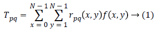
By projecting an image f(x,y) of size N × N on to a set of Tchebichef polynomial kernel, image moment (otherwise called Tchebichef moment) can be computed. The two basic attributes of DTM are order s and degree n, where order s=p+q. The moment Tpq (p,q=0,1,2,…,N-1) is defined as
Where rpq(x,y) is the Tchebichef kernel function expressed as
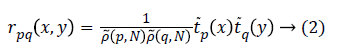
Here, ![]() is the scaled Tchebichef polynomial of degree n.
Sampling grid defined by each Tchebichef polynomial kernel
rpq(x,y) of specific order, when projected on the given image
f(x,y) assess correlation between the image and the respective
kernel. Higher magnitude of Tpq implies high correlation. Both
the spatial and frequency domain representation of these
kernels for N=8 is shown in Figure 2. With N=8, possible
orders are s=0,1,…,2N-2 and total number of kernels are 64.
Order 0 has only one kernel which is r00alone. Order 1 is
constructed from 2 kernels namely r01;r10. Similarly for N=8,the maximum counts of kernels that contribute to the order s=7
is high and are r70,r07,r61,r16,r52,r25,r43,r34. A texture signature
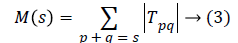
can be constructed as proposed by Macros [29] as
is the scaled Tchebichef polynomial of degree n.
Sampling grid defined by each Tchebichef polynomial kernel
rpq(x,y) of specific order, when projected on the given image
f(x,y) assess correlation between the image and the respective
kernel. Higher magnitude of Tpq implies high correlation. Both
the spatial and frequency domain representation of these
kernels for N=8 is shown in Figure 2. With N=8, possible
orders are s=0,1,…,2N-2 and total number of kernels are 64.
Order 0 has only one kernel which is r00alone. Order 1 is
constructed from 2 kernels namely r01;r10. Similarly for N=8,the maximum counts of kernels that contribute to the order s=7
is high and are r70,r07,r61,r16,r52,r25,r43,r34. A texture signature
can be constructed as proposed by Macros [29] as

Figure 2: (a) Spatial and (b) Frequency domain representation of Tchebichef kernels for N=8.
The number of kernels k that contribute M(s) is defined as
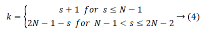
DTM feature vector can be formed in many ways. Typical one proposed by Macros [29], as expressed in equation 3 consists of 2N-1 features. In the proposed work feature vector is constructed from all the individual kernels for which p=q. This corresponds to all those kernels running in the diagonal from top left to bottom right. With N=32, the number of features that contribute feature vector of a sample becomes 32.
Support vector machine
Extracted features are given to a classifier to carry out the classification task using supervised learning scheme. Support Vector Machines are statistical supervised learning model that comes under machine learning strategy often employed to solve classification and regression tasks. With a set of training samples, SVM training algorithm builds a model that categorizes the unknown samples into any one of the two classes using hyperplanes. A hyperplane that has the largest margin to the nearest training data serves as a good separating plane and the SVM operates on those hyperplanes, hence, has less classification error compared to other classifiers. SVMs can efficiently perform non-linear classification by mapping the finite dimensional input space samples into a high dimensional feature space using kernel tricks. Some common kernels used in SVM are Linear (dot product), Gaussian radial basis function, Polynomial etc. The basic SVM classifier is a binary classifier but, real world classification tasks are often multi class nature. However, to make a binary classifier to work with multi class tasks two classic schemes are employed namely one-versus-all (OVA) and all-versus-all (AVA). In the proposed work, OVA scheme has been employed using MATLAB. It involves training a classifier by keeping one class alone as positive and all the rest as negative. Such an approach decomposes the multi class problem into a binary problem and then the basic SVM is applied. It should be repeated for the number of classes.
In the proposed work, a sample is formed by grouping two blocks one from the parenchyma block (whose block size is 32 × 32) and another one from the renal sinus block (whose block size is 16 × 16). Feature extraction is carried out using Discrete Tchebichef Moment, where the feature vector is constructed from all the individual DT kernels for which p=q. Hence, a total of 48 features (32 features constructed from the parenchyma and 16 from the renal sinus.) constitute the feature vector. To accomplish training and testing, samples are bifurcated into two sets. Training and testing samples are chosen randomly and a 5 fold cross validations has been used to study the experimental result. To avoid domination of one attributes over the other, attributes are scaled before fed into the classifier. The proposed method is shown in Figure 3.

Figure 3: Proposed CAD system.
Experimental Works and Discussion
In the present study, ultrasound kidney images as described in section 3 have been used. 4 non overlapping parenchymal regions (size 32 × 32) and 4 central regions (size 16 × 16) have been marked in each image by the radiologist. With 40 images, this result in a total of 160 samples for this proposed study. The samples representing the parenchyma and the renal sinus region belonging to the four different classes are shown in Figure 4 respectively. Discrete Tchebichef moments are extracted from these regions to construct the feature vector. The features extracted from the parenchymal region and the renal sinus region are concatenated to form a single vector of size 1 × 48. From the available 160 samples, a feature matrix is constructed by taking the samples (160) in the row, and their corresponding features (48) in the column resulting in a 160 × 48 matrix. The respective class labels are organized as a 160 × 1 matrix. These samples are subjected to random split and a k fold cross validation procedure has been adapted to obtain the training set and testing set. A multiclass SVM that works on one versus all is utilized to carry out multiclass SVM implementation. The random choice of choosing the testing and training samples with k fold cross validation is repeated 50 times to assess the accuracy of the proposed model.

Figure 4: Column 1to 4 Samples from parenchymal regions; Columns 5 to 8 Renal sinus region. Row1-Hydronephrosis; Row2- Nephrocalcinosis; Row-3 Normal; Row-4 Multicystic.
Classification accuracy is the ratio of number of correct predictions made by a classifier divided by the number of total predictions carried out [30]. Classification accuracy alone cannot be accepted as a measure for the performance of a classifier in situations where, the samples selected for the training as well as testing did not possess equal numbers from each of these classes. It’s a usual practice to evaluate precision and recall measures for individual classes that uses the confusion matrix. Precision and recall measures of the ith class can be given as
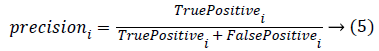
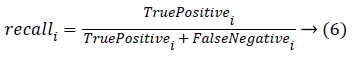
The overall precision and recall measures are nothing but the average of all the precision and recall obtained with individual classes. Robustness of the classifier can be studied by repeating the k-fold cross validation for n number of times. Hence, accuracy, precision and recall measures for the individual class, overall precision and over all recall are estimated and are tabulated for the 10 trials in Table 1. In Table 1, C1, C2, C3 and C4 corresponds to the four classes of kidney considered in this study i.e., Hydronephrosis, Nephrocalcinosis, Normal and Multi cystic dysplasia respectively.
| S. No | Accuracy | Precision | Recall | Overall | |||||||
|---|---|---|---|---|---|---|---|---|---|---|---|
| C1 | C2 | C3 | C4 | C1 | C2 | C3 | C4 | Precision | Recall | ||
| 1 | 90.63 | 0.7872 | 1 | 0.9523 | 0.9032 | 0.925 | 1 | 1 | 0.7 | 0.9107 | 0.9062 |
| 2 | 90 | 0.8182 | 0.9523 | 0.9 | 0.8823 | 0.9 | 1 | 1 | 0.75 | 0.9007 | 0.9 |
| 3 | 90 | 0.8085 | 0.9743 | 0.9512 | 0.8787 | 0.95 | 0.95 | 0.975 | 0.725 | 0.9032 | 0.9 |
| 4 | 91.25 | 0.8182 | 1 | 0.9523 | 0.8823 | 0.9 | 1 | 1 | 0.75 | 0.9132 | 0.9125 |
| 5 | 89.38 | 0.8085 | 0.95 | 0.95 | 0.8787 | 0.95 | 0.95 | 0.95 | 0.725 | 0.8968 | 0.8938 |
| 6 | 88.75 | 0.8372 | 0.9714 | 0.9512 | 0.7948 | 0.9474 | 0.85 | 0.975 | 0.775 | 0.8886 | 0.8868 |
| 7 | 89.38 | 0.8222 | 1 | 0.9523 | 0.8108 | 0.925 | 0.9 | 1 | 0.75 | 0.8963 | 0.8938 |
| 8 | 88.12 | 0.7826 | 0.974 | 0.9512 | 0.8235 | 0.9 | 0.95 | 0.975 | 0.7 | 0.8829 | 0.8813 |
| 9 | 90.63 | 0.8181 | 0.9756 | 0.9512 | 0.8823 | 0.9 | 1 | 0.975 | 0.75 | 0.9068 | 0.9063 |
| 10 | 89.38 | 0.8095 | 0.9756 | 0.9512 | 0.8333 | 0.85 | 1 | 0.975 | 0.75 | 0.8924 | 0.8924 |
Table 1. Performance metrics of proposed method.
A slightly deviated model that employs DTM features that belongs to the highest order alone has been chosen to extract the image moments. Such a highest order includes all those kernels running in the diagonal from top right to bottom left in the spatial/frequency domain representation in Figure 2. For N=32, the highest order kernels count to 32. Similarly for the renal sinus region, the block size chosen is 16 × 16 i.e N=16. For this case, the number of features counts to 16. Thus the total number of features, counts to 48 in this approach. Same SVM classifier is adapted with 5 fold cross validation to assess the performance of the proposed method. Results obtained with 50 trials are averaged and the average overall precision and recall are estimated. F-Score is nothing but the harmonic mean of overall Precision and overall Recall. Comparative results are tabulated as Method 1 in Table 2.
| S. No | Name of the Method | Accuracy | Overall Precision | Overall Recall | F-Score |
|---|---|---|---|---|---|
| 1 | Proposed Method | 0.8916 | 0.8916 | 0.8929 | 0.8922 |
| 2 | DTM Method1 | 0.849 | 0.8507 | 0.849 | 0.8498 |
| 3 | DTM with only Parenchyma region | 0.5477 | 0.5397 | 0.5477 | 0.5436 |
| 4 | Hu’s Feature | 0.7165 | 0.7359 | 0.7165 | 0.7264 |
| 5 | GLCM Feature | 0.7369 | 0.7373 | 0.7369 | 0.737 |
Table 2. Classification results with 5 different feature extraction techniques.
A study that involves only the parenchyma region has also been studied to prove the importance considering both the parenchyma region and renal sinus region of the proposed method. Considering only the parenchyma region seems to be quite simple and the number of features extracted from this region is only 32. The same 160 samples with k fold cross validation results are found. Results obtained with 50 trials are averaged and the average overall precision and recall are tabulated as DTM based method 2 in Table 2.
Study that involves the use of seven invariant moments proposed by Hu is also compared. Hu’s moments are popular for their invariance to rotation, translation and scaling. These seven moments for the parenchyma region whose block size is 32 × 32, as well as for the renal sinus region whose block size equal to 16 × 16 are extracted. A total of 14 features are extracted to represent each sample. Feature vector constructed for the 160 samples each represented with 14 features gives rise to a 160 × 14 matrix. Multi class SVM classifier with k fold cross validation is utilized to assess the performance of the model. Results obtained with 50 numbers of trials are averaged and tabulated as Hu’s method in Table 2.
A quite primitive and frequently used feature extraction method is Gray Level Co- occurrence matrix (GLCM). GLCM approach takes into account the relative position of the pixel with respect to its neighbour in estimating the feature. Hence, to compare the performance of the proposed method, a study using the GLCM is also conducted. GLCM matrix for two different offsets is found for the two blocks. GLCM features such as autocorrelation, correlation, contrast, energy, entropy, homogeneity and dissimilarity are found. This gives rise to 28 features per sample. Feature matrix is constructed with 160 samples each have 28 features. Multi class SVM classifier with k fold cross validation is utilized to assess the accuracy of the model. Results obtained with 50 numbers of iterations are averaged and tabulated as GLCM method in Table 2.
Table 1 reveals that normal kidney can be distinguished from the abnormal one almost accurately which can be revealed from the high score of C3. The high precision for the normal kidney implies that the system returns substantially more relevant results than irrelevant. Mis-classification seems to be high between hydronephrosis and multi cystic dysplasia. This is, because the renal sinus echo patterns of these two classes are more relevant when hydronephrosis is severe. In some cases, Multi cystic dysplasia showed some overlap with the nephrocalcinois due to the high acoustic enhancement that happens just beneath the cyst. The images available in the database have different levels of severity in their respective classes hence showed a little misclassifications. The Table 2 reveals that discrete Tchebichef Moment based features outperforms the rest in terms of accuracy, overall precision, overall recall and fscore. This can be realized with the high scores obtained with the proposed method as well as from the DTM Method 1 when compared to the rest. When the proposed method (i.e DTM) is tried with the parenchymal block alone, the result became very poor which isrevealed from row 3 of Table2. Proposed method and DTM method 1 showed good results of more than 0.85. GLCM feature based method as well as Hu’s moment based feature extraction when fed into the multi class SVM gives little low result compared to the proposed method.
According to the experts, the images utilized in the study can be easily classified by an expert radiologist, and the system performances are little low as per their perspective. This is because, the attributes utilized in this study are highly limited compared to a practical scenario and the features such as shape, size and patient body conditions are not taken into consideration while carrying out the classification task.
Conclusion
This paper demonstrates the applicability of DTM features in classifying the echo patterns of four categories of ultrasound kidney images with the aim of implementing computer aided classification in ultrasound B-mode kidney images. Since discrete orthogonal moment possess non redundant, easy implementation, less computation attributes, propoesed feature extraction is implemented using DTM. Effectiveness of DT moments in extracting features are experimentally demonstrated. A multi class SVM with One vs All scheme with RBF kernels have been used to carry out the classification. Quantitative evaluation of the proposed method is done using Accuracy, Precision and Recall measures of individual class as well as with overall precision recall and fscore estimation. Comparative analysis of the proposed method is carried out with the popular feature extraction schemes such as Hus moment and GLCM feature based methods. Experimental results reveal the efficiency of the proposed method in kidney disorder classification compared to the rest. Further works can be carried out by including other attributes like shape and size of the kidney and patient body conditions to realize a CAD in practice.
Acknowledgement
Authors would like to acknowledge the radiologist Dr. Diravidamani and Sonologist Dr. Jay for their help in collecting the database and carrying out the manual segmentation of organ and as well as marking the parenchyma region and renal sinus region utilized in this study. Also, authors would like to thank their respective management and principal for their support in carrying out this research.
References
- Cerrolaza JJ, Otero H, Yao P, Biggs E, Mansoor A, Ardon R, Jago J, Peters CA, Linguraru MG. Semi-automatic assessment of pediatrichydronephrosis severity in 3D ultrasound. SPIE Med Imaging IntSoc Optics Photon 2016.
- Doi K. Computer-aided diagnosis in medical imaging: historical review, current status and future potential. Comput Med Imaging Graphics 2007; 31: 198-211.
- Chen CM, Yi-Hong C, Tagawa N, Do Y, Computer-aided detection and diagnosis in medical imaging. Comput Math Methods Med 2013.
- Johnson RJ, Feehally J, Floege J. Comprehensive clinical nephrology. Elsevier Health Sci2014.
- Chen DR, Yi-Hsuan H. Computer-aided diagnosis in breast ultrasound. J of Med Ultrasound 2008; 16: 46-56.
- Ayer T, Ayvaci MU, Liu ZX, Alagoz O, Burnside ES. Computer-aided diagnostic models in breast cancer screening. Imaging Med 2010; 2: 313-323.
- Junji S, Sugimoto K, Moriyasu F, Kamiyama N, Shiraishi J, DoiK.Computer-aided diagnosis for the classification of focal liver lesions by use of contrast-enhanced ultrasonography. Med Phys2014; 35: 1734-1746.
- Singh N, Jindal A. A segmentation method and comparison of classification methods for thyroid ultrasound images. Int J Comput App 2012; 50: 43-49.
- Sugimoto K, Shiraishi J, Moriyasu F, Doi K. Computer-aided diagnosis for contrast-enhanced ultrasound in the liver. World J Radiol 2010; 2: 215-223.
- Ulagamuthalvi V, Sridharan D. Automatic identification of ultrasound liver cancer tumor using support vector machine. IntConfEmerg Trends Comput Electron Eng 2012.
- Ho CY, Tun-Wen P, Yuan-Chi P, Chien-Hung L, Yung-Chih C, Yang-Ting C,Kuo-Su C. Ultrasonography Image Analysis for Detection and Classification of Chronic Kidney Disease. IntConf Complex Intel Software Intensive Sys, 2012 Sixth International Conference 624-629. IEEE.
- Pujari RM, Hajare VD. Analysis of ultrasound images for identification of Chronic Kidney Disease stages. International Conference on Networks & Soft Computing (ICNSC- 2014) 380-383, IEEE.
- Bommanna Raja K, Madheswaran M, Thyagarajah K. A hybrid fuzzy-neural system for computer-aided diagnosis of ultrasound kidney images using prominent features. J Med Syst 2008; 32: 65-83.
- Attia MW, Abou-Chadi FEZ, El-Din Moustafa H, Mekky N. Classification of Ultrasound Kidney Images using PCA and Neural Networks. IJACSA 2015; 6: 53-57.
- KohilavaniE, ThangaselviE,RevathyO. Analysis and classification of ultrasound kidney images using texture properties based on logical operators. Int J EngTechnol2012; 2: 750-755.
- AkkasaligarPT,Birandar S. Classification of Medical Ultrasound images of Kidney. IJCA online proceedings on International Conference on Information and Communication Technologies ICICT 2014; 3: 24-28.
- Subramanya MB, Kumar V, Mukherjee S, Saini M. SVM-Based CAC System for B-Mode Kidney Ultrasound Images. J Digit Imaging 2015; 28: 448-458.
- Quaia E. Radiological Imaging of the kidney, 2nd Ed, 2011, Springer, Berlin, Germany.
- Bama S, Selvathi D. Despeckling of medical ultrasound kidney images in the curvelet domain using diffusion filtering and MAP estimation. Signal Processing 2014; 103: 230-241.
- MukundanR, Ramakrishnan K. Moment functions in Image analysis; Theory and Applications. 1998, World Scientific Publishers, Honkong.
- Hu MK. Visual pattern recognition by moment invariants. IRE Transact InformaTheor1962; 8: 179-187.
- Liao SX, Pawlak M. On image analysis by moments. IEEE Transact Pattern Anal Machine Intell 1996; 18: 254-266.
- Papakostas GA. Over 50 Years of Image Moments and Moment Invariants. Moments Moment Invariants-Theor App 2014; 3-32.
- Teague MR. Image analysis via the general theory of moments. JOptical Soc Am 1980; 70: 920-930.
- Mukundan R, Ong SH, Lee PA. Image analysis by Tchebichef moments. IEEE Trans Image Process 2001; 10: 1357-1364.
- Mukundan R, Ramakrishnan K. Local Tchebichef Moments for Texture Analysis. UC Research Repository, 2014.
- Yap PT, Paramesran R, Ong SH. Image analysis by Krawtchouk moments. IEEE Trans Image Process 2003; 12: 1367-1377.
- Zhu H, Shu H, Zhou J, Luo L, Jean-Louis C. Image analysis by discrete orthogonal dual Hahn moments. Pattern RecognitLett 2007; 28: 1688-1704.
- Víctor MJ, Cristóbal G. Texture classification using discrete Tchebichef moments. J Optic Soc Am 2013; 30: 1580-1591.
- Sokolova M, Guy L. A systematic analysis of performance measures for classification tasks. Inf Process Manag2009; 45: 427-437.