ISSN: 0970-938X (Print) | 0976-1683 (Electronic)
Biomedical Research
An International Journal of Medical Sciences
Research Article - Biomedical Research (2017) Volume 28, Issue 3
Classification of EEG signals for wrist and grip movements using echo state network
Brain-Computer Interface (BCI) is a multi-disciplinary emerging technology being used in medical diagnosis and rehabilitation. In this paper, different techniques of classification and feature extraction are applied to analyse and differentiate the wrist and grip flexion and extension for synchronized stimulation using sensory feedback in neuro-rehabilitation of paralyzed persons. We have used an optimized version of Echo State Network (ESN) to identify as well as differentiate the wrist and grip movements. In this work, the classification accuracy obtained is greater than 96% in a single trial and 93% in discrimination of four movements in real and imagination.
Keywords
Brain computer interface, EEG signal, Limb movements, Emotiv, Rehabilitation, ESN.
Introduction
The popularity of analysing brain rhythms and its applications in healthcare is evident in rehabilitation engineering. Motor disabilities as a consequence of stroke require rehabilitation process to regain the motor learning and retrieval. The classification of EEG signals obtained by using a low cost Brain Computer Interface (BCI) for wrist and grip movements is used for recovery. Using Movement Related Cortical Potential (MRCP) associated with imaginary movement as detected by the BCI, an external device can be synchronized to provide sensory feedback from electrical stimulation [1]. The timely detection, classification of movement and the real time triggering of the electrical stimulation as a function of brain activity is desirable for neuro-rehabilitation [2,3]. Thus, BCI has an active role in helping out the paralyzed persons who are not able to move their hand or leg [4]. Using BCI system, EEG data is recorded and processed. The acquired data should have the least component of environmental noise and artifacts for effective classification [5]. EEG signals acquired from the invasive method are found to exhibit least noise components and higher amplitude. However, in most applications, a non-invasive method is preferred. The human brain contains a number of neuron networks. EEG provides a measurement of brain activity as voltage fluctuations which are recorded as a result of ionic current within neurons present inside the brain [6]. Many people have motor disabilities due to the nerve system breakdown or accidental failure of nerve system. There are different methods to resolve this problem, e.g. neuro-prosthetics (neural prosthetics) and BCI [3,7-9]. In neuro-prosthetics, a solution of the problem is in the form of connecting brain nerve system with the device and in BCI connecting brain nerve system with computer [2]. BCI produce a communication between brain and computer via EEG, ECOG or MEG signals. These signals contain information of any of our body activity [10]. Moreover, in addition to neuro-rehabilitation, assistive robotics and brain control mobile robots also utilizes similar technologies as reported recently [11,12]. The signal processing of these low amplitude and noisy EEG signals require special care during data acquisition and filtering. After recording EEG measurements, these signals are processed via filtration, feature extraction, and classification. Simple first or second order Chebyshev or Butterworth filter can be used as a low pass, high pass or a notch filter. Some features can be extracted by using one of the techniques from time analysis, frequency analysis, time-frequency analysis or time-space-frequency analysis [13,14]. Extracted EEG signal further classify by using one of the techniques like LDA, QDA, SVM, KNN etc. [15,16].
We aim to classify the wrist and grip movements using EEG signals. This research will be helpful for convalescence of persons having disabilities in wrist or grip. Our work is based on offline data-sets, in which the EEG data is collected multiple times from 4 subjects. We present the following major contributions in this paper: First, the differentiation between the wrist and grip movements has been performed by using imaginary data as well as the real movements. Secondly, we have tested multiple algorithms for feature extraction and classification and used ESN with optimized parameters for best results. This paper is organized as follows: section 2 describes a low-cost BCI setup for EEG, section 3 deals with the DAQ protocol, section 4 explains the echo state network and its optimization while section 5 discusses results obtained in this research. Section 6 concludes the paper.
Brain Computer Interface Design
Brain-Computer Interface (BCI) design requires a multi-disciplinary approach for engineers to observe EEG data. Today, a number of sensing platforms are available which provide a low-cost solution for high-resolution data acquisition. Developing a BCI interface requires a two-step approach namely the acquisition and the real-time processing. In off-line processing, the only requirement is to do the acquisition. The data is acquired via a wireless network from the pick-off electrodes arranged on the scalp of the subjects [17]. One such available system is Emotiv, which is easy to install and use. Emotiv headset with 14 electrodes and 2 reference electrodes, CMD and DRL, is used to collect data as shown in Figure 1. All electrodes have potential with respect to the reference electrode. Emotiv headset is a non-invasive device to collect the EEG data as preferred in most of the diagnosis and rehabilitation applications [18].

Figure 1. Emotiv EEG acquisition using P-300 standard.
It is important to understand the EEG signal format and frequency content for pre-processing and offline classification. Table 1 shows some of the indications of physical movements and mind actions associated with different brain rhythms in somewhat overlapping frequency bands. It is obvious that the motor imagery tasks are associated with the μ-rhythm in 8-13 Hz frequency band [19].
| Rhythm | Frequency (Hz) |
Indication | Diagnosis |
|---|---|---|---|
| Δ | 0-4 | Deep sleep stage | Hypoglycaemia, Epilepsy |
| υ | 4-7 | Initial sleep stage | - |
| α | 8-12 | Closure of eyes | Migraine, Dementia |
| β | 12-30 | Busy/Anxious thinking | Encephalopathies, Tonic seizures |
| γ | 30-100 | Cognitive/motor function | - |
| µ | 8-13 | Motor imagery tasks | Autism Spectrum Disorder |
Table 1. Brain frequency bands and their significance.
Data Acquisition Protocol
Data is recorded for real and imaginary movements. Firstly, the wrist real movement data of right hand is recorded followed by the grip movement and then imaginary movement data is recorded for wrist and grip in the same scenario as shown in Figure 2 and Figure 3 respectively. Data protocol is designed for data recording [25]. The protocol is illustrated in Figure 4. After the raw data is collected, a 4th order Butterworth filter is applied. A rectangular window is applied with an overlap to make small data sets. Classification and feature extraction techniques are applied to classify the data.

Figure 2. Wrist movement [25].

Figure 3. Grip movement [25].

Figure 4. Data acquisition protocol.
Initially, the subject is at calm position, and data recording protocol video is started as follows:
1. Subject is at rest while EEG data recording is started.
2. EEG data recorded for relax position for 5 seconds.
3. Wrist flexion EEG data recorded for 5 seconds.
4. Calm time for 3 seconds.
5. Wrist extension EEG data record for 5 seconds.
6. Calm time for 3 seconds.
7. Wrist flexion EEG data recorded for 5 seconds.
8. Process continued for 60 times of EEG data recording.
A total of 60 trials from each subject, with 921 samples of 5 sec each were recorded. Data collection electrodes are shown in fig 1, while motor cortex position is shown as highlighted electrodes on skull [26]. Let’s assume that we have data E (t), and this dataset is segmented into small segments by windowing as in Equation 1. In our case the rectangle window with t=921 samples is used.
y(t)=E(t)*rect(t)→(1)
There are challenging issues to handle the EEG signals in order to recognize different tasks. First of all, the EEG signals have a non-stationary pattern. Secondly, these signals have no specific single pattern change which can be used to recognize a specific task. To sum up, the human random task classification makes it more difficult in the presence of noise and artifacts [27].
To overcome these problems; different signal processing techniques, classifiers, and feature extraction algorithms are used to recognize the specific tasks [7,8,19,24,28]. Many research papers have been found to report algorithms for different EEG classification tasks as shown in Table 2.
| Technique | Task | Result | Ref |
|---|---|---|---|
| ESN | Wrist and finger movement imagery | 71% | [20] |
| PNN | Emotion | 91.33% | [21] |
| BPNN | Imagine movement of right, left-hand movement | 85% | [22] |
| PNN | Cortical potential cursor move | 90% | [23] |
| ESN | Song, fist, rotate cube, Count |
Single trial 95% Four task 65% |
[24] |
Table 2. Results with neural network variants.
The offline classification task flow is shown in Figure 5. Pre-processing is important to remove biases and noise from the data. Before the feature extraction step, the data is passed through referencing, filtering and signal enhancement stages. The reference electrode should be placed where signal strength is zero. In our case, the common reference electrodes are used near the ear lobes for a zero potential.

Figure 5. Block diagram of off-line classification.
Topo plots for grip and wrist movement
Motor cortex plots for right-hand wrist and grip movement are shown in Figures 6 and 7. Rejection method encompasses discarding contaminated EEG based on automatic or visual inspection while subtraction encompasses the hypothesis that the contaminated EEG contains a linear combination of original EEG and the artifact.

Figure 6. Topo plot for wrist movement.

Figure 7. Topo plot for grip movement.
Filtration and windowing
After acquiring the raw data, it is processed through the windowing and filtration. For filtration, a band pass filter of 0.2-128 Hz is used with 512 Hz sampling frequency [29]. Fourth order Butterworth filter is used to remove the line noise of 48-52 Hz. Windowing of signals is done after the filtration for feature extraction. Chebychev and Gaussian window is applied on the data set of size 52 × 1 with a step size of 0.1 s.
Feature translation
Feature extraction is related to the dimensionality reduction in the sense that it transforms the high dimensional data to a lower dimension. Choice of the method depends on the type of BCI system, band power, Power Spectral Density (PSD), time-frequency representation, Hjorth parameters, etc. For the linear dimensional reduction technique, Principle Component Analysis (PCA) is preferred as it maps the data linearly in such a way that the variance in low dimensional data maximizes.
Power spectral density method is used as a feature [4]. Band power is the best discriminant between the imagination based movement data. It falls within the alpha and beta bands with frequency ranges comprising of 9-14 Hz and 18-26 Hz.
Classification results
For classification purpose, techniques used include the radius basis function SVM, Quad SVM, QDA, LDA and the Naive Bayesian with normal distribution [15,30-32]. As a linear discriminant classifier, we used LDA, while for the non-linear classification; Naive Bayes with normal distribution is used. These classifiers are applied on EEG datasets after pre-processing and filtering. Results of these classifiers are finally compared with an Echo State Network (ESN) with optimized parameters. A brief description of these classifiers is as follows:
Linear discriminant analysis (LDA): In LDA, classification of the different datasets is obtained via training and testing the given dataset. The confusion matrix is used to quantify the performance of the classification method. Performance is evaluated on testing the dataset on the basis of given results. Confusion matrix can be explained with the example. Let’s start with binary classification. In binary classification, the dataset is divided in two sets which are analysed on the basis of occurrence of specific task. The confusion matrix is shown in Table 3.
| N=No. of dataset | Predict “action 1” | Predict “action 2” |
|---|---|---|
| Actual “action 1” | TN | FP |
| Actual “action 2” | FN | TP |
Table 3. Confusion matrix representation.
The symbols presented in the above table are illustrated as follows:
True negative (TN): Prediction of movement is “Move Up” and actual result is also “Move Up”.
True positive (TP): Prediction of movement is “Move Down” and actual result is also “Move Down”.
False negative (FN): Prediction of movement is “Move Up” and actual result is not “Move Up”.
False positive (FP): Prediction of movement is “Move Down” and actual result is not “Move Down”.
As an example, if we have 100 datasets of wrist movement, in which 50 datasets are for the case when wrist is “move up” and 50 for the “move down” case, confusion matrix is constructed as shown in Table 4.
| N=100 | Predict “Move up” |
Predict “Move Down” |
|---|---|---|
| Actual “Move up” | 40 | 10 |
| Actual “Move Down” | 8 | 42 |
Table 4. Confusion matrix example.
In this example as shown in Table 4, the prediction for up and down movements, is shown , where 40 samples shows up-movement while 10 shows that these doesn’t occur. On the basis of this classification, following results are evaluated.
Accuracy of the classifier is described as:
Accuracy = (TP+TN)/Total number of samples.
Error Rate represents the un-classified data. It is defined as:
Error Rate = (FP+FN)/Total number of sample.
Error Rate = 1-Accuracy.
Sensitivity Rate shows the case when both prediction and actual results are matched, i.e. Sensitivity = TP/Actual Yes.
False Positive Rate depicts the mismatch between the actual and prediction.
False positive Rate = FP/Actual No
Specificity is the case when both prediction and actual results are “No”.
Specification = TN/Actual “No”
Precision is achieved when prediction and actual result match.
Precision = TP/Predict “Yes”
Prevalence, when matched form occurs mostly is given as:
Prevalence = Actual Yes/Total
This explanation is summarized in Table 5.
| N=100 | Predict “Move up” | Predict “Move Down” | |
|---|---|---|---|
| Actual “Move up” |
40 | 10 | Actual Yes (50) |
| Actual “Move down” |
8 | 42 | Actual No (50) |
| Predict “Yes” (48) | Predict “No” (52) |
Table 5. Confusion matrix explanation.
The experiment is executed for four subjects from where a number of EEG datasets are recorded. After collecting EEG datasets, whole signals are segmented. Then, these segments are passed through the filters. In the present case, we used Butterworth filter with Nyquist rate of 512 Hz. After filtration, features are extracted from the dataset. These features help to classify the data. As showed in Table 6. Then, LDA is applied for classification from where the confusion matrix is recovered.
| ESN iteration |
Hidden layers | Accuracy% |
|---|---|---|
| I | 50 | 88.39 |
| II | 70 | 97.23 |
| III | 90 | 97.85 |
| IV | 100 | 96.14 |
| V | 120 | 93.55 |
| VI | 140 | 91.71 |
| VII | 160 | 90.32 |
| VIII | 200 | 88.43 |
Table 6. Dependence of ESN accuracy on no. of hidden layers.
Quadratic discriminant analysis (QDA): After accomplishing the result from LDA, QDA is applied on the EEG datasets. QDA is an advanced version of LDA. The part of the QDA classifier that contrasts from the LDA classifier is the calculation of the discriminant functions. The LDA discriminant functions are a simplified version of the QDA ones, arrived at by using a single average covariance matrix and dropping identical terms on all sides of the comparison [33]. In practice, the calculation is simplified to being linear in terms of x, instead of quadratic. The results are recorded in Table 7. Both the Hjorth activity and mobility parameters were used.
| Movement | Signal | Classifier | Accuracy% |
|---|---|---|---|
| Real vs. Imaginary movement | Wrist | LDA | 44.23 |
| QDA | 52.64 | ||
| NB | 41.59 | ||
| ESN_op | 93.06 | ||
| Real vs. Imaginary movement | Grip | LDA | 49.52 |
| QDA | 71.63 | ||
| NB | 56.25 | ||
| ESN_op | 96.07 | ||
| Real movement | Wrist Vs. Grip |
LDA | 68.99 |
| QDA | 77.64 | ||
| NB | 65.38 | ||
| ESN_op | 95.69 | ||
| Imaginary movement | Wrist Vs. Grip |
LDA | 46.63 |
| QDA | 50.96 | ||
| NB | 36.30 | ||
| ESN_op | 93.50 |
Table 7. Comparison of classification results.
Naive bayesian (NB): In Naïve Bayes method, the probability of the most probable class is established. The probability of each of the instance of the class is found which have an unseen instance. So, Bayesian classifier can be described as follows:
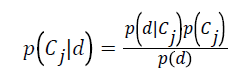
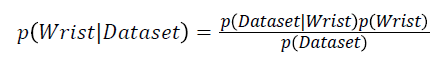
Where, p (Cj | d) is the probability of instance “d” which is in class Cj and p (d | Cj) is the probability of generating class at instance “d” for a given class Cj. p (Cj) is the probability of occurrence. P (d) is the probability of occurance of instance “d”, so, in this equation, we want to compute the probability of “d” which is is p (d | Cj) in the class Cj. Also, the probability of having some feature in ‘d’ with the imagined probability is p (d | Cj). Applying these concpets to the problem in hand, suppose if we want to classify hand wrist and grip movements, initially, there is no resource to distinguish this type of movement. So, in Bayes method, the probability of data is a concern. We can say that testing datasets are grip or wrist movements. It can be represented as in form of wrist testing:
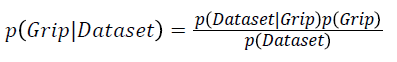
And for the grip testing,
This probability can be accessed via training dataset. In training, the probability is made on the basis of feature vectors that are extracted after the filtration and segmentation. So, final Bayes is made as follows:
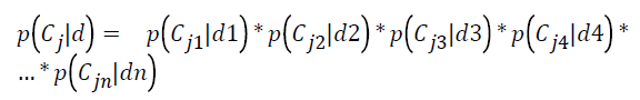
Naïve Bayes classification results are also presented in Table 7.
Echo-state Network for Classification
In machine learning, several different algorithms are in practice. Artificial Neural Networks (ANN) and its variants e.g. Feed-Forward Neural Networks (FFNN) and discrete-time Recurrent Neural Networks (RNN) are some of the most popular black-box modelling techniques in learning and classification. Due to the limitations of RNN; as a result of their complexity, computationally expensive training requirements and difficulty in analysing lot of efforts were concentrated towards simple approaches resulting in the development of Echo State Network (ESN) [10]. It has been reported that ESN fits in most of the situations by just modifying the tuning parameters [34]. Also, it performs well in the presence of artifacts. The classification steps in ESN learning algorithm are shown in Figure 8.

Figure 8. ESN classification steps.
ESN is a supervised learning algorithm, in which there is a training input signal

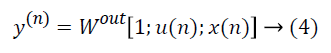
Where, n = 1, 2 …T and ‘T’ is the total number of data set. Initially, weights are assigned randomly and after that, they are updated with training data set. So, we call them input and recurrent weights, these are Win ε RNx∞(1+Nu) and W ε RNx × Nx. With the training data set, reservoir set is made named x (n). Linear readout weight Wout is computed from the reservoir set, which minimizes the Mean Square Error (MSE). Finally, the input data set is applied to final readout weights to compute output y (n).
Reservoir data set is made with the following equation,
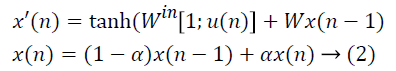
Hyperbolic tangent function is used as follows:
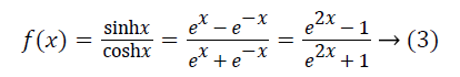
This hyperbolic tangent function is found to be more helpful for the training data set as compared to the sigmoid function. This is because of the reason that when a negative input is applied it goes into indeterminant state, while hyperbolic tangent function works in a deterministic manner.
Network output is y (n) ε RNy, which is:
Some of ESN parameters are as follow:
• Output is linear neuron (linear system is useful for complex and multivariate signals)
• Alpha (α) represents a smoothing factor that is a non-negative number. A larger value represents a higher smoothing factor.
• Eigenvalues are used as the weights of the dynamic reservoir. These eigenvalues are used to train the dataset.
• Finally, weights calculated on behalf of pseudo-inverse and output weights are updated.
Eigenvalues are used to distinguish or to determine any change in signal. First, the training is processed using no-motion data and its eigenvalues are saved. In the second step, these eigenvalues are applied on input dataset to analyse any change.
Single electrode output is examined by this method and results are acquired. Figure 9 shows the original sequence and the output of the ESN.

Figure 9. ESN for network output.
After completing work on single electrode, results are made to discriminate the different movements. The classification results are presented in Table 7.
Results and Discussion
The classification results are shown in Table 7 where a comparison is presented between the LDA, QDA, NB and ESN_op algorithms for different movement types. For the real vs. imaginary movement of the wrist and grip, it has been found that on average, LDA and NB classifiers are showing closer accuracies on the lower side while the QDA is better classifying the movements as compared to the previous two.
On the other hand, ESN_op is showing the best accuracy in both cases with accuracy above 90%. In comparing classification of the real and the imaginary movements data of both wrist and grip movements, it has been found that the LDA and NB perform well for the former case, however for the latter case, poor accuracies have been obtained. Likewise, the QDA accuracy also drops for the classification of imaginary wrist and grip movements. ESN_op also shows a slight degradation in accuracy from 95.69% to 93.50% for imaginary movements. Perhaps, due to relatively lower information in imaginary data, rest of the algorithms show degraded performance. But as the ESN_op is a novel, noise redundant and robust algorithm, its performance still dominates. Respective accuracies are obtained by calculating the confusion matrices for the classifiers.
Conclusion
This paper describes an offline task classification for wrist and grip movements in both imagination and real movements. The classification is required in order to perform rehabilitation using brain computer interface technology. Both wrist and grip movements using real and imaginary data is used for the classification. Several algorithms are used on the same data while optimizing few of them for best possible depiction of results. It has been found that the parameter Optimized ESN (ESN_op) is performing the classification task with highest accuracy as compared to LDA, QDA and NB. In future, the online data will be used to detect real time movements using this algorithm. The challenge of real time classification involves less complexity of the algorithm on one side while a high performance and computationally efficient hardware on the other side. We are targeting to achieve both in our future research while using a High Performance Computing (HPC) platform in our lab. Multichannel EEG data will be processed and results will be available with less than a microsecond time delay. A high performance multicore embedded architecture is in the development phase for real-time protocol implementation.
References
- Pfurtscheller G, Muller-Putz GR, Scherer R, Neuper C. Rehabilitation with brain-computer interface systems. Comp 2008; 41: 58-65.
- Mrachacz-Kersting N, Jiang N, Dremstrup K, Farina D. A novel brain-computer interface for chronic stroke patients. Br Comp Interf Res Springer 2014; 51-61.
- Xu J, Haith AM, Krakauer JW. Motor control of the hand before and after stroke. Clin sys neurosci Springer 2015; 271-289.
- Mashal F, Shafique M, Khan ZH. Towards a low cost brain-computer interface for real time control of a 2 DOF robotic arm. Int Conf Emerg Technol IEEE 2015.
- Kubler A, Leeb R, Neuper C, Muller D. Combining brain computer interfaces and assistive technologies state-of-the-art and challenges. Front Neurosci 2010; 4: 1-15.
- Ghulyani S, Pratap Y, Bisht S, Singh R. Brain computer interface. Brain 2012; 1.
- Valbuena D, Cyriacks M, Friman O, Volosyak I, Graser A. Brain-computer interface for high-level control of rehabilitation robotic systems. Rehabilitation Robotics 2007; 619-625.
- Xu K, Mai J, He L, Yan X, Chen Y. Surface electromyography of wrist flexors and extensors in children with hemiplegic cerebral palsy. PM R 2015; 7: 270-275.
- Zhou J, Yedida S. Channel selection in EEG-based prediction of shoulder/elbow movement intentions involving stroke patients: a computational approach. Comp Intel Bioinf Comput Biol 2007; 455-460.
- Kathner I, Ruf CA, Pasqualotto E, Braun C, Birbaumer N. A portable auditory P300 brain-computer interface with directional cues. Clin Neurophysiol 2013; 124: 327-338.
- Bell CJ, Shenoy P, Chalodhorn R, Rao RP. Control of a humanoid robot by a noninvasive brain-computer interface in humans. J Neural Eng 2008; 5: 214-220.
- Gergondet P, Druon S, Kheddar A, Hintermüller C, Guger C, Slater M. Using brain-computer interface to steer a humanoid robot. Robo Biom 2011; 192-197.
- Mak JN, McFarland DJ, Vaughan TM, McCane LM, Tsui PZ. EEG correlates of P300-based brain-computer interface (BCI) performance in people with amyotrophic lateral sclerosis. J Neural Eng 2012; 9: 026014.
- Lee H, Cho S. Pca+ hmm+ svm for eeg pattern classification. Signal processing and its applications. Proc Int Symp IEEE 2003; 541-544.
- Alomari MH, Samaha A, AlKamha K. Automated classification of l/r hand movement eeg signals using advanced feature extraction and machine learning 2013.
- Bashashati H, Ward RK, Birch GE, Bashashati A. Comparing Different Classifiers in Sensory Motor Brain Computer Interfaces. PLoS One 2015; 10: e0129435.
- Cincotti F, Mattia D, Aloise F, Bufalari S, Schalk G. Non-invasive brain-computer interface system: towards its application as assistive technology. Brain Res Bull 2008; 75: 796-803.
- Javaid MA. Brain-Computer interface 2013.
- Jochumsen M, Niazi IK, Dremstrup K, Kamavuako EN. Detecting and classifying three different hand movement types through electroencephalography recordings for neurorehabilitation. Med biol eng comp 2015: 1-11.
- Mohamed AK, Marwala T, John LR. Single-trial EEG discrimination between wrist and finger movement imagery and execution in a sensorimotor BCI. Eng Med Biol Soc EMBC 2011; 6289-6293.
- Murugappan M, Murugappan S. Human emotion recognition through short time Electroencephalogram (EEG) signals using Fast Fourier Transform (FFT). Sig Proc Appl IEEE Int Col 2013; 289-294.
- Dan X, Zhengdong M, Jianfeng H. A linear discrimination method used in motor imagery eeg classification. Natural Comput 2009; 94-98.
- Huaping J. Neural network in the application of EEG signal classification method. Comput Intel Secur 2011; 1325-1327.
- Forney EM, Anderson CW, Gavin WJ, Davies PL, Roll MC, Taylor BK. Echo state networks for modelling and classification of EEG in mental task Bci 2014.
- Fatima M, Shafique M, Khan D, Hussain N. Feature extraction of EEG signals using wireless data acquisition system.Ieep Conf 2015.
- Wang Y, Hong B, Gao X, Gao S. Phase synchrony measurement in motor cortex for classifying single-trial EEG during motor imagery. Eng Med Biol Soc 2006; 75-78.
- Lai W, Huosheng H. Towards multimodal human-machine interface for hands-free control. A surv 2011.
- Shuman G, Duric Z, Barbara D, Lin J, Gerber LH. Using myoelectric signals to recognize grips and movements of the hand. Bioinf Biomed 2015; 388-394.
- Suleiman ABR, Fatehi TAH. Features extraction techniques of EEG signal for BCI applications. Electr Eng Uni Mousl 2007.
- Omari FA, Liu G. A novel prosthetic hand classification approach using libSVM classification method. J Info Opt Sci 2015; 36: 183-195.
- Wairagkar M, Daly I, Hayashi Y, Nasuto S. Novel single trial movement classification based on temporal dynamics of EEG 2014.
- Vidyasagar KC, Moghavvemi M, Prabhat T. Performance evaluation of contemporary classifiers for automatic detection of epileptic EEG. Industr Instr Contr 2015; 372-377.
- Uktveris T, Jusas V. Comparison of feature extraction methods for EEG BCI classification. Info Softw Technol Springer 2015; 81-92.
- Lukosevicius M. A practical guide to applying echo state networks. Neu Netw Trade Springer 2012; 659-686.