ISSN: 0970-938X (Print) | 0976-1683 (Electronic)
Biomedical Research
An International Journal of Medical Sciences
Research Article - Biomedical Research (2017) Volume 28, Issue 7
Assessment of a novel computer aided mass diagnosis system in mammograms
Omid Rahmani Seryasat and Javad Haddadnia*
Department of Electrical and Computer Engineering, Hakim Sabzevari University, Sabzevar, Iran
- *Corresponding Author:
- Javad Haddadnia
Department of Electrical and Computer Engineering
Hakim Sabzevari University
Sabzevar, Iran
Accepted on December 7, 2016
Mammography is the most common modality for screening breast cancer. In this paper, a computer aided system is introduced to diagnose benignity and malignancy of masses. In the first step of the proposed method, masses are prepared for segmentation using a noise reduction and contrast enhancement technique. Afterward, a region of interest is segmented using a new adaptive region growing algorithm, and boundary and texture features are extracted to form its feature vector. Consequently, a new robust architecture is proposed to combine weak and strong classifiers to classify masses. Finally, the proposed mass diagnosis system was also tested on mini-MIAS and DDSM databases. The accuracy of the obtained results is 93% in the database of MIAS and 90% in the database of DDSM. The obtained results indicate that the proposed system can compete with the stateof- the-art methods in terms of accuracy.
Keywords
Breast cancer, Mammography, Benign, Malignant.
Introduction
Breast cancer is considered an important disease in various countries (especially western countries). According to statistics, breast cancer is the most common cancer after lung cancer (10.9% of cancers in men and women is breast cancer [1]) and is the fifth cause of cancer deaths [2]. The rate of breast cancer has increased in the past decade. However, mortality from cancer among women (of all ages) has declined. This decline is related to the widespread use of medical imaging by means of which radiologists diagnose cancer in early stages [3]. Since statistics shows that 96% of cancers are treatable in the preliminary stages, early diagnosis is the best way to deal with breast cancer [2]. Mammography is the most common method of breast imaging. This method alone has decreased the death rate from breast cancer by as much as 25 to 30 percent [3]. One of the most important symptoms of breast cancer is a mass in mammography. The idea of helping radiologists by means of computer systems is not related to the present. Rather, computer scientists have tried to assist radiologists in the identification and diagnosis of masses nearly in the last three decades. CAD systems aim to aid radiologists in the diagnosis of abnormalities in the images, and the replacement of radiologists with these systems has never been the purpose. There are also other methods such as multi-peak histogram equalization and histogram stretching that removes the equalization defects of the histogram in some cases. The methods based on global histogram equalization are able to enhance the image contrast well. There are also other methods that are based on multi-scale image processing such as wavelet transformation. For the classification of the masses, it is necessary that some features be extracted in order to be distinguishable from the two categories. These features are related to mass intensity, mass texture, mass border and geometric features as well. The features concerning mass intensity are extracted from the statistical information related to mass gray levels in the tumor region. Some information such as minimum and maximum values, mean, variance, skewness and Kurtosis can be placed in this category [4-6]. Generally, a variety of features is extracted in the field of medical diagnostics using computer systems and artificial intelligence. These are evident that among its features there might be a number of additional or irrelevant features, thus they decreases the accuracy of the system. Therefore, feature selection methods can be used for improving the accuracy of the classification. For example, the method of step by step feature selection has been used [7]. In another method offered [8], they combined SVM-RFE method with NMIFS method. The method presented [9] first limits the image to the mass region and changes it to the standard size of 32 × 32. Then, using PCA and ICA transform obtained from training images and the standard basis of Gabor transform, it transfers the image into three different subspaces and uses the visual representation of each of these three subspaces as a category of features. To extract feature vectors, a wavelet transform db4 is applied on ROI up to five levels [10]. Moreover, due to the effect of noise on the first level of transformation, the coefficients of the first level have been excluded. Finally, the energy of each of the normalized transform levels is used as feature vectors [10]. In this paper, we will offer a new strategy for the classification of samples which does not depend on the type of classifier that has been used.
Materials and Methods
In this section, we describe the proposed method in this paper to diagnose what types of masses exist in mammogram images. In the proposed method, first, a series of preprocessing is carried out on the area (ROI) in which the masses are located. At the next stage, the mass is classified and its contour is extracted. Extracting a good contour is critical because benignity and malignity of masses are interrelated with the irregularity of the mass border. From the viewpoint of radiologists, the more irregular a mass border is, and the higher the malignancy of a mass will be. In the next sections, our purpose is to learn the type of classification which is able to diagnose both benignity and malignantly of masses. Then, we investigate each of the existing modules in more details.
In this paper, we have used two different databases including Mini-MIAS and DDSM. The database of Mini-MIAS contains 330 images with 1024 × 1024 resolution [11,12]. These 330 images include only the MLO view of the patient. Of these 330 images, 209 ones are normal which means that they lack any mass, asymmetry, distortion and micro calcification. Of the remaining images, 56 images include at least one mass. One of these 56 images (mdb059) has been excluded in our tests because there is no information of the mass position in that image. There are 58 masses in these 55 tested images, 38 of which are benign and 20 of which are malignant. The database of DDSM is a public database with a large number of images, and researchers usually select a subset of that and perform their tests. There are both MLO and CC views for each patient in this database. This database has been compiled by different scanners and bit depths. In this paper, we have selected from this database 120 images with benign masses and 120 images with malignant masses.
Pre-processing
The aim of the pre-processing is to reduce the noise of mammograms and to enhance the edges of the mass. In this step, median filtering with the 3 × 3 window is used as the noise reduction method. Then, to increase the contrast of the ROI Equation 1 is utilized. Figure 1 illustrates the impact of this pre-processing approach.
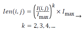 (1)
(1)

Figure 1. Impact of pre-processing approach.
Mass segmentation
On one the most important steps are classifying masses is boundary extraction because its irregularity is considered as a measure of malignancy. In this paper, an adaptive automatic region growing algorithm is used to extract mass boundary. In the first step of this algorithm, the region of interest is divided into 32 × 32 non-overlapping blocks. Then, sum average feature is extracted from each block based on the constructed GLCM matrix. For applying region growing two important questions arise 1) where is the location of seed point 2) what is the homogeneity measure. In the proposed method, the seed is the pixel with highest sum average feature. For the second question, region grows until the estimated radius of the region is close to the ground truth radius of that as much as possible. Note that ground truth radius is estimated by radiologists and it is available in the databases. Figure 2 illustrates some examples of applying the proposed segmentation method.

Figure 2. Examples of applying the proposed segmentation method.
Feature extraction
Feature extraction plays an important role in identifying models, and selection of suitable features enhances the classification accuracy. These features should be able to reveal similarities between objects in a class and at the same time they should able to show the difference of those objects with the ones in other classes. Generally, the features that are extracted to identify the type of masses can be divided into two groups: 1. Textural features 2. Morphological features.
Morphological features: We used boundary features based on normalized radial length [13,14] as morphological features. The coordinates of the masses should be identified in order to determine the features associated with mass border. Accordingly, two criteria including radial length and coordinates-border are defined.
Radial length: To calculate the (Normalized Radial Length) NRL, the coordinates of the center of mass is first obtained. Then, the Euclidean distance of points in the border from the center of mass is measured and finally normalized.
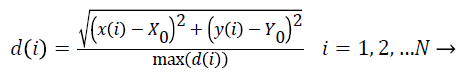 (2)
(2)
In the above equation, (X0,Y0) are the coordinates of the center of mass, (x (i), y (i)) are the coordinates of the points on the border in i place , N is the total number of points on the border and max (d (i)) is the maximum radial length which has been extracted. The features defined based on the radial length include:
1. Average NRL:
The average normalized radial length represents the expansion of the mass in the tissue and somehow also refers to the size of the tumor:
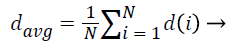 (3)
(3)
2. The standard deviation of NRL:
The standard deviation of radial length is another criterion that somehow indicates the extent of changes in radial length in mass and thus determines the irregularity in the mass and branching of borders.
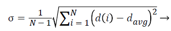 (4)
(4)
3. Roughness index:
Roughness Index is a criterion for calculating the roughness of the mass borders and indicates the changes in radial length from any point on the border to its neighbouring point and in some way determines the irregularity and branching of the border [15].
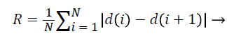 (5)
(5)
4. Zero crossing:
Zero crossing is calculated based on the number of times the radial distance obtained from the border areas is equal to the average radial distance. Therefore, in addition to showing border branching and irregularity, it indicates the number of lobes on the border.
5. Moments of boundary:
This criterion examines the structures of micro boundaries and the extent of their branching and it is obtained by the following equation. Lower-order moments can be used for less sensitivity to noise.
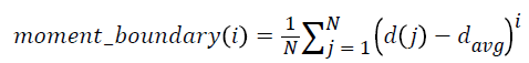 i = 1, …, 5 → (6)
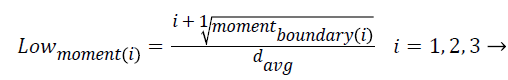 (7)
(7)
6. Fourier shape descriptor:
Fourier Shape descriptor (FDM) is obtained by deriving the Fourier transform from the bounding coordinates and normalizing it. The frequency components represent the boundary points and describe how the boundary behaviour changes.
FD=fft (bounding coordinates) → (8)
FDM=FD/(abs (FD (1, 1))) → (9)
Based on this definition and a statistical analysis, the following features can be defined:
Mean_FDM: the average Fourier Shape descriptor function
Variance_FDM: the amount of variance of Fourier Shape descriptor function
Energy_FDM: the amount of energy of Fourier Shape descriptor function
Entropy_FDM: the amount of irregularity of Fourier Shape descriptor function
Textural features: When a mass has a more heterogeneous and rougher tissue, the likelihood of mass malignancy also increases. In this paper, features based on empirical mode function are used to describe the texture of the masses [17]. EMD is a decomposition method of any compound data set into a finite and often small number of components which are known as Intrinsic Mode Functions (IMF) [18,19]. This method can be used for analysing nonlinear and non-stationary data. If EMD is used for analysing image texture, it is known as BEMD. BEMD, considering basic concept of EMD, uses steps which will be defined as follows:
Step 1) Reading the input data image, I (x, y). Initializing h (x, y)=I (x, y);
Step 2) Finding out all the extreme points in data.
Step 3) Joining all the maximum points for obtaining the upper envelope U (x, y) and join the entire minimum points for getting the lower envelope L (x, y) through the help of surface interpolation.
Step 4) Find out the average value m (x, y) of upper and lower envelope as given in Equation 10,
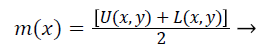 (10)
(10)
Step 5) Subtracting this average value from h (x, y), and check whether the obtained value h (x, y) satisfies the condition of an IMF or not, as shown in Equation 11.
h(x,y)=h(x,y)-m(x,y) → (11)
If that the total number of extrema and the number of zero-crossings is either be equal or differ at most by one, it would be the first condition of an IMF. During the second condition, at each point, the mean value of the envelope defined by the local maxima and the envelope defined by the local minima will be zero.
Step 6) (a) in the case of not happening h (x, y) as an IMF, treat it as an original data and repeat steps 1 to 5 until the first IMF is found. The process of finding an IMF is known as a sifting process. As it is given in Equation 12, stopping criterion of this sifting process, that is a value of SD, is chosen between 0.2 and 0.3.
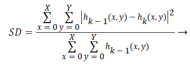 (12)
(12)
Step 6) (b) if the IMF is found by h (x, y), then it is known as first IMF. IMF1=h (x, y) and then r (x, y)=I (x, y)-IMF1. Check whether r (x, y) is monotonic or not. If it is monotonic then it would be a residue and no more IMF can be extracted, and if it is not a residue, it would be treated as an original signal and it would be repeated all the steps discussed above. After finding all the IMFs we will get the original data through superimposing them and adding residue in that as in Equation 4, where n is the total number of IMFs.
In this paper, BEMD has been applied for extracting features on preprocessed ROIs, and two IMFs have been obtained for each ROI. IMFs are two-dimensional matrices (size of each IMF is 40 × 40) so that the size of the feature vector for all images will be very large cause’s classification very complicated and time-consuming. Therefore, five statistical parameters of mean, standard deviation, skewness, kurtosis, and entropy had been extracted from these coefficients in order to reduce the size of the feature vector.
Classification
This section deals with one of the most important innovations of this paper which are designing and implementing a novel ensemble classifier. Basically, designing ensemble classifiers is based on the principle of diversity. This means that diversity somehow should be created in the basic classifiers that have been used. This diversity creation can be carried out at 4 levels: 1. Data level 2. Feature level 3. Classifier level 4. Combiner level. Creating diversity at data level means that the basic classifiers use different samples such as Bagging and Ada Boost in order to be trained. Diversity at feature levels indicates that all basic classifiers are not to be trained in a fixed set of features and should use a different set of features for training including rotation forest. The third level is based on the principle that we should use different professional classifiers for training. In fact, the classifiers whose training methods are different should be used. The last level is related to combiner level. For example, a variety of strategies like majority votes weighted voting and using a learner can be combined in order to create diversity. In this paper, we aim to offer a new strategy for the combination. In this section, we will describe the suggested architecture to create a new ensemble classifier. The purpose is to diagnose the samples that are easily classified by uncomplicated classifiers (with a little flexibility and fewer features) and diagnose difficult samples by more complex classifiers (by considering more features for samples). As you know, the training error decreases when a more complex classifier is used. However, the testing errors might increase and generalizability might decrease. In fact, the gap between training and testing errors increases. In fact, according to the principle of occum's razor, of the competing hypotheses, the hypothesis that has fewer assumptions is better. Hence, the simplicity of an important principle lies in generalization. Simpler systems usually have higher generalizability. In order to reduce this gap, an adaptive architecture has been suggested, according to which the complex classifiers will be used only for difficult samples rather than for simple ones. For this purpose, we suggest the following block diagram shown in Figure 3.

Figure 3. Block diagram of adaptive architecture.
We first start from the testing stage for an easier explanation. A sample is introduced to our system in order to determine the benignity or malignancy. This sample is given to AdaBoost1. AdaBoost1 is a classifier that determines the malignancy with confidence and on the other hand, AdaBoost2 confidently diagnoses benign samples. In fact, Ada Boost has a default threshold on zero. If the amount of support obtained for a sample is positive, the sample is malignant and if it is negative, it is benign. To create a reliable classifier which is able to diagnose malignant samples (AdaBoost1), the threshold should increase. As for AdaBoost2, however, the threshold should decrease. When a sample is difficult (the simple whose benignity and malignancy cannot be confidently diagnosed by simple classifiers), other strategies should be used in order to increase the classification power of the classifier. For example, more features can be extracted instead of that difficult sample (increasing dimension) or the flexibility of the classifier can be enhanced. For example, if we use SVM, we can enhance the flexibility of the classifier by exploiting a more complex kernel. It should be noted that we can use other classifiers such as Naive Bayes instead of Ada Boost and achieve our goals by changing their threshold. We also take advantage of this strategy in this paper and from all the features consider only a subset of them for simple classifiers. Nonetheless, we will use the samples with all their features for complex classifiers. At the training stage, we will use 10-fold-cross validation strategy on the training set to determine whether the samples are easy or difficult. In fact, we create other training sets and tests from the training set. According to this strategy, 90% of the samples will be used for training and the remaining will be used for testing (validation) in each testing. To put it simply, consider the first frequency of the 10 possible frequencies. In this frequency, 10% of the set is used for testing and the remaining 90% is used for training. We train the simple classifiers with this 90%. Now consider 10% of the testing set. We test these two simple classifiers on the samples of this set. In the case of making incorrect or less confident prediction about a sample, the sample is added to the training set of the complex classifier. Now let’s consider the second frequency. The second 10% of the set is used for testing and the rest is used for training and we separate the difficult samples from the second testing set according to the above-mentioned statement. We continue this process until the tenth frequency. The training set of the complex classifier is prepared after identifying the difficult samples in the whole training set. Therefore, we train the complex classifier in the set which has been prepared.
Results
In this paper, we have used 10-fold cross validation strategy 5 times for the steps of tests and results, and all the results related to the classification step are based on the mean of these five tests. As for the adjustment method of these parameters and other ones in the section of machine learning, we use 90% of the training set in 10-fold strategy as the validation set. In fact, we carry out another 10-fold cross validation on that 90% for parameter adjustment. This strategy is considered a standard method for the adjustment of relevant algorithm parameters in machine learning. To evaluate the efficiency of mass classification, the following criteria which are obtained by confusion matrix as shown in Table 1 are usually used:
Accuracy=(TP+TN)/(TP+FP+TN+FN) → (13)
FNR=FN/(FN+TP) → (14)
FPR=FP/(FP+TN) → (15)
Sensitivity=TP/(TP+FN) → (16)
Specificity=1-FPR= TN/(TN+FP) → (17)
| Predicted class | |||
|---|---|---|---|
| Actual class | Malignant-class | Benign-class | |
| Malignant-class | a (TP) | d (FN) | |
| Benign-class | b (FP) | c (TN) | |
Table 1. Confusion matrix.
In the above equations, TP, TN, FP, and FN are the abbreviations for true positive, true negative, false positive and false negative, respectively. Accuracy indicates to what extent the relevant classifier has classified the items correctly. In addition, FPR and FNR show false positive rate and false negative rate. As a matter of fact, these two criteria represent the system error. The false positive rate which is sometimes called false alarm rate as well indicates what percent of benign masses have been incorrectly classified as malignant ones. False negative rate also suggests that what percent of malignant masses have been incorrectly classified as benign ones by the classifier. We adjusted our parameters in validation set so that FNR would be fewer than FPR. In the real world also the cost of these two errors is not the same and FNR is more important than FPR because a patient may die if a malignant mass is mistakenly classified as a benign mass as shown in Table 1. However, if a benign mass is identified as a malignant one, the patient is sent to pathology. In this case, the patient incurs more stress and cost. In fact, it can be said that the issue of classification is a cost-sensitive issue. This cost-sensitivity can be introduced to classification method in different ways but we do not discuss it since this issue is not the purpose of this paper. One of the well-known criteria that are used by most medical diagnostic systems for evaluating the efficiency of their classification is the area under the ROC curve, a curve based on the sensitivity of specificity that is achieved by changing the threshold decision. The closer this number is to 1, the higher the efficiency of the classifier will be. In Table 2, a brief comparison has been made between the proposed method in this paper and other methods. But it should be noted that the accurate comparison is not possible in this case since different methods do not usually use the same data and strategy for their tests and due to the fact that there are no benchmark standards in this regard. As you can see in Table 2, the efficiency of the system considerably increases if the proposed feature selection method is used. In addition, the proposed method will result in fewer false negative rates, compared to the false positive rates. In addition, in the proposed method we can reach higher areas under the ROC curve by using the appropriate feature selection method. Unfortunately, a false negative rate which is the most important error criterion has not been reported in most systems. Fortunately, however, the error criterion of false negative rate is low in our system to such an extent that it reached only 1% on the mini-MIAS database.
| Database | Accuracy (%) | FPR (%) | FNR (%) | AUC | |
|---|---|---|---|---|---|
| Proposed classifier | MIAS | 93 | 14.5 | 1 | 0.94 |
| Proposed classifier | DDSM | 90 | 12 | 7.5 | 0.93 |
| Mu et al. [1] | MIAS | - | - | - | 0.92 |
| Rojas et al. [2] | DDSM | 81 | - | - | - |
| Rangayan et al. [3] | MIAS | - | - | - | 0.82 |
| Tahmasbi et al. [4] | MIAS | 93.6 | 8.2 | 3.2 | - |
| Rangayan et al. [5] | MIAS | 81.5 | - | - | 0.7 |
Table 2. Comparison of our proposed method with other competing methods in terms of accuracy; FPR: False Positive Rate; FNR: False Negative Rate; AUC: Area Under ROC Curve.
Discussion
One of the most effective ways to detect breast cancer, especially in the early stages, is mammography. One of the ways to combat this disease is to diagnose it in the early stages. According to most of the physicians, if the cancer is detected in its early stages, more effective treatments can be done and the probability of the mortality rates will be reduced. Studies show that Imaging mammography in women without symptoms periodically greatly reduces cancer rates. In this investigation, a series of mammography images have been processed based on a standard database.
In this study, some patients with digital mammography images and with minimal missing data have been handled. One of the most important innovations of this paper is to improve a general and efficient framework for clustering benign and malignant samples. In this article, Boosting algorithm has been used as the base classification. However, other algorithms can be applied. For example rotation forest and random forest as well as other compound categories can be used. This method of classification is applied as a second interpreter by the radiologists and its purpose is helping to radiologists in identifying benign and malignant mass. By no means, the aim of developing of such systems is replacing them instead of specialists, but this system helps the radiologists. Zhao et al. in their research [17] used the harmonic and fuzzy filter to remove noise. Khan et al. [18], use K-Means cluster to remove impulsive noise. But this method is both complex and timeconsuming and these were the weaknesses of their method. |In our proposed method, the median filter with size 3 × 3 has been used to remove and improve noise. Then, techniques for increasing contrast have been used in the image. Evaluation results indicate better performance and superiority of the proposed approach compared to last proposed methods for detection and removal of impulsive noise, detect and recover textures and edges of the image and quality of image noise.
Authors recognized and segmented malignant tumors in mammographic images by using multi-stage thresholding and improving the image [19]. Although the proposed algorithm [19] follows from a simple algorithm and it has good diagnostic accuracy. However, its size and computational time are very high due to a large number of fields of the mammographic image that should be processed locally and its problems have been corrected in proposed method in our paper. In fact, more degrees of freedom can be provided for radiologists by using the proposed framework. This degree of freedom is applying Thresholding on the output of clustering algorithms. Since the output of classification is probability, therefore, radiologists can achieve thresholding on this probability output to achieve true positive rate and false positive. This freedom of action is among the positive features of assistance systems. In other words, the radiologist themselves can apply the desired threshold, between the two mentioned rates. As we know, the true positive rate and the false positive rate are in conflict with each other. Authors clustered images by using 14 proposed features and support vector machine, while, and in our proposed method the number of features has decreased [20]. Authors adopted Gabor filter bank and removed distortion before step clustering in mammogram images [21]. However, the sensitivity of the proposed method was 84% .That in our paper; this value was 93% by the choice of convenient features.
Conclusion
In this paper, a computer aided diagnosis system as a second interpreter is proposed for helping radiologists to classify mass type (malignant or benign). This system achieves an area under the curve of 0.94 and 0.93 for mini-MIAS and DDSM databases, respectively. The novelties of the proposed system can be summarized as presenting a new automatic adaptive region growing algorithm to extract boundary of masses, using descriptors based on empirical mode functions, and introducing a new framework for combining classifiers. Limitations in the proposed model include the failure to provide the extracted features for classification that may not become a good and correct answer in some cases on the offered features. This problem may be due to the nature of the mammogram image of the sample. The proposal that can be suggested for future is using deep neural networks to classify the mammographic image as benign and malignant mass. Neural networks are used widely due to the learning capability of hybrid features in all fields of classification. Deep networks are models of developed neural network for learning nonlinear transformation on the data. On the other hand, a fundamental difference between deep network models with neural networks is that in each layer try to preserve their ability to construct data, which is a distinctive character in mammography.
References
- Hill TD, Khamis HJ, Tyczynski JE, Berkel HJ. Comparison of male and female breast cancer incidence trends, tumor characteristics, and survival. Ann Epidemiol 2005; 15: 773-780.
- de Oliveira JEE, de Albuquerque AA, Deserno TM. Content-based image retrieval applied to BI-RADS tissue classification in screening mammography. W J Radiol 2011; 3: 24.
- Oliver I Malagelada A. Automatic mass segmentation in mammographic images: Universitat de Girona 2007.
- Huang NE, Shen Z, Long SR, Wu MC, Shih HH, Zheng Q. The empirical mode decomposition and the Hilbert spectrum for nonlinear and non-stationary time series analysis. Proc Royal Soc London Math Phys Eng Sci 1998.
- Ghafarpour A, Zare I, Zadeh HG, Haddadnia J, Zadeh FJS, Zadeh ZE. A review of the dedicated studies to breast cancer diagnosis by thermal imaging in the fields of medical and artificial intelligence sciences. Biomed Res 2016.
- Kim JK, Park JM, Song KS, Park HW. Adaptive mammographic image enhancement using first derivative and local statistics. IEEE Trans Med Imag 1997; 16: 495-502.
- Surendiran B, Vadivel A. Feature selection using stepwise anova discriminant analysis for mammogram mass classification. International J Rec Trend Eng Technol 2010; 3: 55-57.
- Liu X, Tang J. Mass classification in mammograms using selected geometry and texture features, and a new SVM-based feature selection method. IEEE Sys J 2014; 8: 910-920.
- Costa DD, Campos LF, Barros AK. Classification of breast tissue in mammograms using efficient coding. Biomed Eng 2011; 10: 1.
- Mousa R, Munib Q, Moussa A. Breast cancer diagnosis system based on wavelet analysis and fuzzy-neural. Exp Sys Appl 2005; 28: 713-723.
- Kozegar E, Soryani M, Minaei B, Domingues I. Assessment of a novel mass detection algorithm in mammograms. J Cancer Res Ther 2013; 9: 592-600.
- Mu T, Nandi AK, Rangayyan RM. Classification of breast masses using selected shape, edge-sharpness, and texture features with linear and kernel-based classifiers. J Digit Imaging 2008; 21: 153-169.
- Rojas-Domínguez A, Nandi AK. Development of tolerant features for characterization of masses in mammograms. Comput Biol Med 2009; 39: 678-688.
- Rangayyan RM, Nguyen TM. Fractal analysis of contours of breast masses in mammograms. J Digit Imaging 2007; 20: 223-237.
- Tahmasbi A, Saki F, Shokouhi SB. Classification of benign and malignant masses based on Zernike moments. Comput Biol Med 2011; 41: 726-735.
- Rangayyan RM, Mudigonda NR, Desautels JL. Boundary modelling and shape analysis methods for classification of mammographic masses. Med Biol Eng Comput 2000; 38: 487-496.
- Xiao L, Li C, Wu Z, Wang T. An enhancement method for X-ray image via fuzzy noise removal and homomorphic filtering. Neurocomput 2016; 195: 56-64.
- Khan A, Waqas M, Ali MR, Altalhi A, Alshomrani S, Shim S-O. Image de-noising using noise ratio estimation, K-means clustering and non-local means-based estimator. Comp Electr Eng 2016.
- Dominguez AR, Nandi AK. Enhanced multi-level thresholding segmentation and rank based region selection for detection of masses in mammograms. IEEE Int Conf Acoust Speech Sign Proc 2007.
- Domínguez AR, Nandi AK. Toward breast cancer diagnosis based on automated segmentation of masses in mammograms. Patt Recogn 2009; 42: 1138-1148.
- Ayres FJ, Rangayyan RM. Reduction of false positives in the detection of architectural distortion in mammograms by using a geometrically constrained phase portrait model. Int J Comp Assist Radiol Surg 2007; 1: 361-369.