ISSN: 0970-938X (Print) | 0976-1683 (Electronic)
Biomedical Research
An International Journal of Medical Sciences
Research Article - Biomedical Research (2017) Volume 28, Issue 9
An application of fuzzy normalization in miRNA data for novel feature selection in cancer classification
1Department of Information and Communication Engineering, Anna University, Chennai, India
2Department of Computer Science & Engineering, Bannari Amman Institute of Technology, Sathyamangalam, Tamil Nadu, India
- *Corresponding Author:
- Anidha M
Department of Information and Communication Engineering
Anna University, India
Accepted on February 27, 2017
Feature selection and classification of microarray data are the most important challenges in machine learning. The motivation behind the Feature selection techniques is in selecting discriminate feature subsets which plays a vital role in the process of classifying cancer/tumour microarray expression data. In the present work, a novel feature selection approach is employed which combines F-Score and Relevant Information Gain (RIG) in miRNA data normalized by fuzzy Gaussian membership function. The F-score is employed to identify the discriminative features. The RIG is computed based on the class specific features of mean score values of the features. The experiments are conducted on seven miRNA datasets to demonstrate the performance of a proposed algorithm using the classifiers Support Vector Machine (SVM) and Artificial Neural Network (ANN). The experimental results show that the proposed approach gives a better classification accuracy compared to the state-of-the art feature selection algorithms. The proposed feature selection method gives 100% average classification accuracy with SVM and ANN for the Angulo_DI miRNA dataset and higher average classification accuracy for the other datasets compared to existing feature selection methods.
Keywords
Feature selection, miRNA microarray, Relevant information gain, Classification.
Introduction
Microarray technology is used to monitor thousands of gene expression levels simultaneously and is considered to be central in the recent years. Identifying significant feature based on expression levels becomes an essential for diseases prognosis and diagnosis. Microarray technology accelerates the analysis of thousands of miRNA expression profiles simultaneously. Several studies have recently demonstrated that miRNA expression profiles represent a useful tool for deciphering the genetic basis of malignant diseases. The miRNA expression profiles are highly reproducible among different patient cohorts that suggest a possible application as diagnostic biomarkers [1].
miRNAs play important regulatory roles in many cellular processes, including differentiation, neoplastic transformation, and cell replication and regeneration. Because of these regulatory roles, it is not surprising that aberrant miRNA expression has been implicated in several diseases. The recent studies have reported significant levels of miRNAs in serum and other body fluids by raising the possibility that miRNAs could serve as useful clinical biomarkers [2]. However, the most challenging issue in this high dimensional data analysis is a huge number of features and a small number of samples. One important issue is to find the marker genes [3]. Marker genes are genes whose expression values are biologically useful for determining the class of the samples. In other words, marker genes are genes that characterize the tumor classes. The identification of marker genes is important due to the following reasons:
• Improves the classification performance
• Provides better biological insights and interaction of relevant genes to achieve certain significant biological and molecular decisions.
• Studies the functional, sequential and molecular behaviour of known marker genes in order to facilitate the functionality and interaction of other genes.
• Allows further study on relation of expression values of different genes with respect to the tumor class and its similar expression pattern always results in cancer or the combination of suppression of certain genes and expression of certain genes are a better indication of tumor, etc [3].
The microarray classification is a two–step process. The first step is to select a subset of significant and relevant features from the set of features and the second step is to develop a classification model that can produce accurate prediction for new data. A true and accurate classification is important for a successful diagnosis and treatment of cancer. The high dimensionality of the DNA microarray data becomes a problem, when it is employed for cancer classification, as the sample size of DNA-microarray is very smaller than the feature size. However, among the large number of features, only a small fraction is effective for performing a classification task. Hence the identification of relevant features is an important task in most microarray data studies that will give higher accuracy for sample classification. This problem can be eased by using machine learning with a feature selection problem. The goal of feature selection methods is to determine a small subset of informative features that reduces processing time and provides higher classification accuracy. There are many potential benefits for feature selection. This include facilitation of data visualization and data understanding, reduces the storage requirements, decreases the training and utilization times and avoids the curse of dimensionality to improve the prediction performance.
In general, the feature selection methods are grouped in to three categories: filters, wrappers and embedded models. Filters are used to score all features in a pre-processing stage and then select the best ones. In wrappers, some feature sets are selected and evaluated via the designed classifiers. The embedded methods, however, are specific to the selected learning machines [4] and the process of feature selection is done in their training step. Some of the common feature selection approaches include: Fischer criterion [5], mRMR method [6], fuzzy entropy [7] and Mutual Information (MI) [8]. Figure 1 shows the three types of feature selection methods.

Figure 1. Feature selection methods.
Traditional approaches select the features for all classes in common though class-specific feature selection algorithms try to identify a subset of features for each class separately. The class-specific feature selection methods that give a better discrimination of classes have been resulted in most of cases [9]. Recently, a few feature selection methods have been proposed which combine fuzzy and other approaches. In this paper, a novel feature selection approach is proposed to identify the relevant features for classification. Initially, the microarray dataset is normalized so that there are no missing values and the data is scaled between specific ranges. The feature values are normalized using fuzzy Gaussian membership function at three levels.
The F-score for individual miRNAs are identified which gives the relevant information about the feature, but the F-score does not reveal the mutual score among the features. Hence, the class specific mean score is computed to identify the central tendency of the features based on the class labels. These scores are used to find the RIG. The proposed method processes each miRNA expression individually to identify the rank of the features. The high rank features are preferred as significant features for classification. The rest of this paper is organized as follows. Section 2 provides the literature review of feature selection. The proposed method for feature selection is described in Section 3. Section 4 presents the experiment results of the proposed method for seven miRNA dataset and the results are compared with state-of-the art feature selection algorithms.
Literature Review
Chronic lymphocytic leukemia [10] is the first known human disease that is associated with microRNA (miRNA) deregulation. Many miRNAs have been found to have a connection with some types of human cancer [11,12]. Therefore, a great deal of research has been done to analyze cancer classification using miRNA expression profiles with machine learning methods. Table 1 shows the methods adopted for classification of miRNA dataset.
| Reference | Topic | Methodology | Dataset |
|---|---|---|---|
| Lu et al. [13] | MicroRNA expression profiles classify human cancers | k-nearest neighbor (KNN) classification method & Probabilistic Neural Network (PNN) algorithm | Bead-based flow cytometric miRNA expression profiling method to analyze 217 mammalian miRNAs from 334 samples |
| Lu et al., Zheng and Chee [13,14] | Cancer classification with microRNA expression patterns found by an information theory approach | Mutual information with entropy | |
| Xu et al. and Lu et al. [13,15] | MicroRNA expression profile based cancer classification using Default ARTMAP | Default ARTMAP for classification & PSO for feature selection | Mammalian miRNA expression profiles |
| Kotlarchyk et al. [16] | Identification of microRNA biomarkers for cancer by combining multiple feature selection techniques | Ensemble methodology | liver, breast, and brain miRNA data |
| Lu et al., Kim and Cho [13,17] | Exploring features and classifiers to classify microRNA expression profiles of human cancer. | Pearson’s and Spearman’s correlation coefficients, Euclidean distance, cosine coefficient, information gain, mutual information and signal to noise ratio used for feature selection and Back propagation neural network, support vector machine, and K-nearest neighbor are used for classification | |
| Ulfenborg et al. [18] | Classification of Tumor Samples from Expression Data Using Decision Trunks | P-score for feature selection and Decision Trunk algorithm for classification | Cancers of the prostate, bladder, breast, and lung, as well as Neuroblastomas. |
| Lu et al. and Li et al. [13,19] | A New Direction of Cancer Classification: Positive Effect of Low-Ranking MicroRNAs | Correlation-based feature selection | |
| Lu et al. and Chakraborty et al. [13,20] | Identifying Cancer Biomarkers From Microarray Data Using Feature Selection and Semi supervised Learning | Kernelized Fuzzy Rough Set (KFRS) and Semi supervised Support Vector Machine (S3VM) | SRBCT, DLBCL, Leukemia |
| Ibrahim et al. [21] | Multi-level gene/MiRNA feature selection using deep belief nets and active learning | Multi-level feature selection approach using deep belief nets and active learning | Prostate cancer, Colon cancer, Ovarian cancer, SRBCT, MLL |
Table 1. Literature Review on miRNA dataset.
Fuzzy logic allows us to properly utilize the information in the uncertainty and fast processing of large bodies of complex knowledge, since processing is performed by numerical computations and not symbolic unification as in, e.g., logic programming formalisms [22]. As opposed to neural nets, fuzzy logic has the advantage that it supports explicit representation of knowledge, like in symbolic formalisms, allowing us to combine knowledge in a controlled way [22]. Elham Chitsaz et al., proposed a new approach based on fuzzy feature clustering which is utilized to select the best features (genes). They have used k-modes, a modified version of kmeans for clustering as a part of Attribute Clustering Algorithm (ACA) [23]. In this method, each feature is assigned to different clusters with different degrees and correlation with each cluster is considered. A feature, which is not, correlated enough with members of one cluster but its correlation among entire clusters is high, gains more chance to be selected in comparison [23].
Tatiana Kempowsky-Hamon et al., proposed a new feature selection algorithm, referred to as MEMBAS for MEmbership Margin Based Attribute Selection which enables to process similarly the three data types (numerical, qualitative, interval) based on an appropriate mapping using fuzzy logic concepts. The algorithm measures simultaneously the contribution of each gene for each of the two classes (Molecular Grade 1 and Grade 3 tumors), in order to find the best discrimination. It extracts the most pertinent markers since it is based on feature weighting according to the maximization of a membership margin [24].
Huerta et al. suggested a fuzzy logic based approach for elimination of information redundancy in microarray data. Initially they fuzzified the data to normalize the expression values and features are grouped based on fuzzy similarity measures. Mutual Information measure is considered to select the informative features in each group [25]. Javier Grande et al., implemented fuzzy mutual information measure to select the relevant features. This algorithm is based on Battiti Algorithm with a discretization pre-process stage [26].
Materials and Methods
Fuzzy logic uses linguistic variables, defined as fuzzy sets, to approximate human reasoning. The proposed feature selection method receives pre-processed high dimensionality microarray data set as an input and produces ranked features based on the combined approach of F-Score and Entropy Based Mean Score on miRNA expression values normalized by fuzzy Gaussian membership function. These top-n miRNAs are used by the SVM and ANN for classification. Figure 2 shows the process of feature selection and validation in the proposed work.

Figure 2. Gene selection and Validation of Proposed Work.
Normalization based on fuzzy Gaussian membership
Fuzzification is the process of transforming crisp inputs into fuzzy values with the help of fuzzy linguistic variables and membership functions. Membership functions are used in both fuzzification and defuzzification processes to map the non-fuzzy (crisp inputs) to linguistic terms and vice versa which quantifies the linguistic terms. The membership functions provide membership values denote degree of membership of a linguistic term.
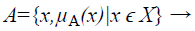
A Fuzzy Set A in the Universe of Discourse X is defined as
 (1)
(1)
Where μA:X → [0,1] with the condition, is the membership function and μA(x) is the membership degree of x in A.
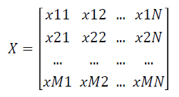
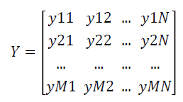
Given a labelled two-class data as an gene expression matrix X with N Features and M Samples as shown below
where xij is the expression value of feature i of jth dimension and i=1 … N and j=1 ... M.
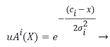
Gaussian fuzzy membership functions are quite popular in the fuzzy logic literature, as they are the basis for the connection between fuzzy systems and Radial Basis Function (RBF) neural networks. The Gaussian membership function applied by using the formula given below in Equation (2):
 (2)
(2)
where mi and σi are centre and width of the ith fuzzy set Ai respectively.
In the fuzzification process, the ideal definition for membership to the set is defined. Each value of the observable fact which is more central to the core of the definition of the set will be assigned as 1. The values that fall between the two extremes fall in the transitional zone of the set, the boundary. As the values move away from the centre of the set, they are assigned a decreasing value on a continuous scale from 1 to 0. The original observable fact has less possibility of being a member of that set since the assigned values decreases. The fuzzification value of 0.5 is the crossover point. Any fuzzy value which is greater than 0.5 indicates the original observable fact may be a member of the set. As the fuzzification values go below 0.5, it is less likely that the original observable fact's value is a member of the set and the values may not be part of the set. Figure 3 depicts the fuzzy Gaussian membership function.

Figure 3. Fuzzy Gaussian Membership Function.
The width of the transition zone depends on the observable fact being modelled. Changing the parameters of the fuzzification function can define the characteristics of the transition zone. Therefore, for Gaussian membership functions with wide widths, it is possible to obtain a membership degree to each fuzzy set greater than 0 and hence, every rule in the rule base fires. Consequently, the relationship between input and output can be described accurate enough. Figure 3 shows the three Gaussian membership functions. The Gaussian membership functions provide more continuous transition from one interval to another and hence provide smoother control surface from the fuzzy rules. Figure 4 portraits the Gaussian membership function at three levels low, medium and high.

Figure 4. Gaussian Membership Function of Three Levels.
For the miRNA expression data set, each attribute values are transformed into fuzzy values by three levels of Gaussian membership values. Initially, the miRNA expression values are arranged in ascending order of the miRNA expression of an attribute and low, medium and high values are identified. All the real values of the miRNA expression eij may belong to one or more levels of Gaussian membership function. The fuzzy value y for each of the Membership functions which eij belongs to is calculated. The y value has to be between 0 and 1. For example: Consider the three membership functions low, medium and high and a given value of eij, and then the degrees of membership to each membership functions (y values) for eij. For example: 0.6 for the membership function low and 0.4 for the membership function medium. Any of the values will belong to at least one membership function with a certain degree of membership. These values are mapped into fuzzy numbers by drawing a line up from the inputs to the input membership functions above and marking the intersection point. The Fuzzy combinations (T-norms) are applied when the value belongs to more than one level of Gaussian membership function.
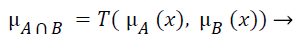
The fuzzy "and" is written as:
 (3)
(3)
where μA is referred as "the membership in class A" and μB is referred as "the membership in class B". There are many ways to compute "and". The two most common are:
Zadeh – min(μA(x),μB(x)). It computes "and" by taking the minimum of the two (or more) membership values.
Product – μA(x) times μB(x) This techniques computes the fuzzy "and" by multiplying the two membership values.
Both techniques have the following two properties:
T(0,0) = T(a,0) = T(0,a) = 0
T(a,1) = T(1,a) = a
The fuzzy expert system transforms the data matrix X which consists of crisp expression values into fuzzy matrix of expression values Y which is represented as follows:
Feature selection using F-Score
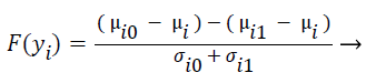
F-score is a mathematical technique which measures the discrimination of two sets of real numbers. Given training vectors yk, where k = 1, ..., M, the F-score of the ith feature is defined as:
 (4)
(4)
where μi ,μi0, and μi1 represent the mean score of feature i, mean score of class 0 of feature i, mean score of class 1 of feature i respectively, and σi0, and σi1 represent the variances of class 0 and class 1 of ith feature respectively. F-Score evaluates the features individually. The numerator indicates the discrimination between the positive and negative sets, and the denominator indicates the one within each of the two sets. The larger the F-score is, the more likely this feature is more discriminative. Therefore, the F-score method is used as a feature selection criterion. A disadvantage of F-score is that it does not deal redundancy among features.
Relevant information gain
The normalized gene expression data Y is converted as matrix S
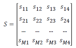
where si1 represents the number of samples in ith gene expression ≥ μi0, si2 represents the number of samples in ith gene expression <μi0 , si3 represents the number of samples in ith gene expression ≥ μi1 and si4 represents the number of samples in ith expression values <μi1.
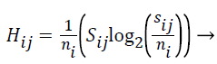
The Entropy values of S are computed using the formula given below:
 (5)
(5)
The Relevant Information Gain (RIG) is computed using the equation (6) to measure the relevance between features and the redundancy among the relevant features.
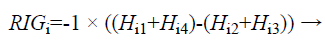 (6)
(6)
The features are ranked (R) using the following formula (7):
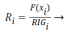 (7)
(7)
Features with high R values are discriminative features and the subset is given as input to the classifiers SVM and ANN.
Experiment Results and Analysis
The datasets used in this study contain expression data for a set of features available at http://sourceforge.net/projects/trunkclassifier/files. These datasets are a part of the collection of database created by Benjamin Ulfenborg, Karin Klinga- Levan and Björn Olsson, Systems Biology research Centre, School of Life Sciences, University of Skövde, Skövde, Sweden [18]. Table 2 shows the description of the dataset.
| Dataset | Cancer | Number of Probes | Class | Total Samples |
|---|---|---|---|---|
| Angulo_DI | Lung | 20185 | Well diff./ Poorly diff. | 51 |
| Takeuchi_SU | Lung | 21619 | Alive/Dead | 149 |
| WangY | Breast | 22283 | ER+/ER- | 286 |
| VandeVijver_SU | Breast | 13359 | Alive/Dead | 295 |
| Sotiriou_GR | Breast | 22283 | Low grade/ High grade | 167 |
| Sotiriou_ER | Breast | 22283 | ER+/ER- | 183 |
| WangQ_ST | Neurobl | 12625 | Early Stage/Late Stage | 101 |
Table 2. Description of the Dataset.
The proposed work is implemented using R version 3.2.4. The datasets are chosen based on the results provided in the previous works. They give less accuracy and contain expression values of miRNAs from cancers of Lung, Breast and Neuroblastomas. Most of the datasets are used for more than one classification tasks such as normal versus malignant and early versus late stage as in Sotiriou Breast cancer data. For breast cancer datasets, histologic grade 1 is considered as low grade and histologic grade >1 as high grade. For neuroblastoma datasets, the International Neuroblastoma Staging System (INSS) stage 1-2 is defined as early stage and INSS stage >2 as late stage [18]. The Wang Y and Sotiriou datasets are log2-transformed before classification [18].
In this work, Support Vector Machine (SVM) and Artificial Neural Network (ANN) are employed as classifiers to identify the performance of feature selection method. The SVM creates a hyper plane or multiple hyper planes in high dimensional space that is useful for classification, regression and other efficient tasks. The SVM constructs a hyper plane in original input space to separate the data points [27]. The overfitting which is avoided by regularization parameter is the advantage of SVM and it uses the kernel trick where the expert knowledge can be built about the problem via engineering the kernel.
An ANN is adaptive in nature because it changes its structure and adjusts its weight in order to minimize the error. An adjustment of weight is based on the information that flows internally and externally through network during learning phase. The advantages of ANN are it requires less formal statistical training, implicitly detect complex nonlinear relationships between dependent and independent variables, detect all possible interactions between predictor variables, and the availability of multiple training algorithms [27].
The classifier performance is evaluated using k-fold cross validation where k as 10. The average accuracy for the given dataset is defined as the proportion of correctly classified test samples
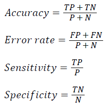
where TP, TN, FP, FN, P and N refer to the number of true positive, true negative, false positive, false negative, positive and negative samples respectively. Table 3 shows the parameters and their values used in the experiment analysis.
The experiment is conducted to identify classification accuracy for different number of features from the ranking list. Table 4 shows the classification accuracy obtained from the classifiers SVM and ANN for top 20, 50 and 100 features. The result shows that for the Takeuchi_SU dataset the accuracy obtained from top 20 features give better result than the result obtained from top 50 features. Both SVM and ANN give least performance for Sotiriou_GR dataset compared to other datasets presented for experiment analysis. The ANN gives the highest classification average accuracy for Angulo_DI, Takeuchi_SU, WangY and Sotiriou_ER datasets. The SVM outperforms for VandeVijver_SU, Sotiriou_GR and WangQ_ST dataset among the three different numbers in miRNAs selection top 100 features outperforms top 20 and top 50 features. So the further analysis is employed for top 100 features.
| Parameter | Value |
|---|---|
| SVM Kernel | Radial Basis Function |
| g | 0.001 |
| Cost | 10 |
| ANN size | 2 |
| Maxit | 1000 |
| Decay | 0.001 |
| k | 10 |
Table 3. Parameters and Values.
| Data Set | Top 20 genes | Top 50 genes | Top 100 Genes | |||
|---|---|---|---|---|---|---|
| SVM | ANN | SVM | ANN | SVM | ANN | |
| Angulo_DI | 90 | 96.7 | 98 | 100 | 100 | 100 |
| Takeuchi_SU | 89.65 | 96.57 | 90.85 | 95.57 | 93.85 | 97.57 |
| WangY | 88.44 | 91.73 | 90.24 | 92.73 | 92.44 | 92.73 |
| VandeVijver_SU | 90.08 | 77.04 | 91.21 | 78.04 | 93.11 | 79.04 |
| Sotiriou_GR | 82.3 | 72.57 | 83.3 | 73.57 | 85.3 | 73.57 |
| Sotiriou_ER | 84.43 | 90.42 | 89.43 | 90.42 | 90.43 | 91.42 |
| WangQ_ST | 90.6 | 81.8 | 96.6 | 80.8 | 99.6 | 82.8 |
Table 4. Classification Accuracy obtained for various number of Top-n genes.
The proposed work gives 100% accuracy for Angulo_DI dataset of Lung Cancer with two states i.e. well differentiated and poorly differentiated for both SVM and ANN. Figures 5 and 6 show the accuracy and error rate obtained from SVM and ANN respectively for top 100 genes.
In addition to cross-validation, the proposed feature selection algorithm is further evaluated using a split sample procedure, where each one of the seven datasets is divided randomly ten times into a training set, containing 50% of the samples, and a test set containing the remaining samples. The average accuracy is taken as accuracy of the classifier. Similarly, the same procedure is applied for 60%-40% and 80%-20%. Table 5 shows the average classification accuracy obtained from the above mentioned partitions. From the experimental analysis it shows that 60%-40% training-testing partition gives better result than the other two partitions 50%-50% and 80%-20%.

Figure 5. Accuracy and Error rate obtained by SVM for top 100 genes.

Figure 6. Accuracy and Error rate obtained by ANN for top 100 genes.
| Data Set | 50%-50% Training-Testing Partitions | 60%-40% Training-Testing Partitions | 80%-20% Training-Testing Partitions | |||
|---|---|---|---|---|---|---|
| SVM | ANN | SVM | ANN | SVM | ANN | |
| Angulo_DI | 97 | 96.7 | 100 | 100 | 98.2 | 98 |
| Takeuchi_SU | 93.65 | 96.57 | 93.85 | 97.57 | 93.85 | 95.57 |
| WangY | 91.44 | 91.73 | 92.44 | 92.73 | 92.44 | 91.53 |
| VandeVijver_SU | 93.05 | 77.04 | 93.11 | 79.04 | 93.11 | 78.04 |
| Sotiriou_GR | 83.3 | 72.57 | 85.3 | 73.57 | 85.3 | 73.57 |
| Sotiriou_ER | 88.43 | 90.42 | 90.43 | 91.42 | 89.43 | 90.88 |
| WangQ_ST | 97.6 | 81.8 | 99.6 | 82.8 | 98.6 | 82.2 |
Table 5. Classification accuracy with various training & test partitions.
Classification accuracies on all datasets of the proposed work as well as all the state-of-the art feature selection algorithms evaluated for comparison are presented in Table 6. It shows that Fuzzy normalized gene expression data has higher average classification accuracy and is the best performing algorithms of all the datasets. The high average classification accuracy is achieved by ANN for the datasets Angulo_DI and Takeuchi_SU for all feature selection methods compared to SVM given in the Table 6. The SVM that gives better performance than ANN for VandeVijver_SU, Sotiriou_GR and WangQ_ST is shown in Table 6. The second and third highest rank of average classification accuracy for SVM and ANN are attained by Mean score and Mutual information.
| Data set | Proposed Method | Mean Score | T-Test | F-Score | SNR | Mutual Information | P-Score [10] | ||||||||
|---|---|---|---|---|---|---|---|---|---|---|---|---|---|---|---|
| SVM | ANN | SVM | ANN | SVM | ANN | SVM | ANN | SVM | ANN | SVM | ANN | SVM | ANN | DTC[10] | |
| Angulo_DI | 100 | 100 | 84 | 88 | 83..2 | 87.8 | 84 | 86 | 80 | 82 | 83.8 | 87.8 | 74.51 | 60.78 | 74.5 |
| Takeuchi_SU | 93.85 | 97.57 | 61.89 | 66.8 | 60.89 | 64.2 | 61.8 | 66.4 | 60.8 | 63.8 | 61.86 | 66.8 | 27.52 | 41.61 | 68.45 |
| WangY | 92.44 | 92.73 | 91.22 | 85.4 | 90.22 | 84.4 | 91.2 | 85 | 90.22 | 83.4 | 90.22 | 85.2 | 86.71 | 87.76 | 89.86 |
| VandeVijver_SU | 93.11 | 79.04 | 73.3 | 71 | 70.3 | 70 | 72.3 | 71 | 70.2 | 69˘.2 | 71.3 | 70.8 | 73.22 | 66.78 | 71.19 |
| Sotiriou_GR | 85.3 | 73.57 | 76.1 | 72.28 | 75.22 | 71.28 | 75.8 | 71.28 | 73.1 | 70.28 | 75.1 | 70.28 | 64.07 | 60.48 | 76.04 |
| Sotiriou_ER | 90.43 | 91.42 | 88.78 | 84.98 | 86.78 | 82.98 | 87.76 | 83.88 | 84.68 | 80.48 | 87.78 | 83.98 | 81.42 | 82.51 | 76.5 |
| WangQ_ST | 99.6 | 82.8 | 87.71 | 81.14 | 86.7 | 80.14 | 85.47 | 81.22 | 80.67 | 78.14 | 86.72 | 79.24 | 72.28 | 82.18 | 83.16 |
Table 6. Comparison of Average Classification Accuracy with Existing Feature Selection Methods.
Receiver Operating Characteristics (ROC) Analysis
Receiver Operating Characteristics (ROC) Curve is used for visualizing the performance of a binary classifier. It is a graphical representation of relationship between sensitivity and specificity. ROC curve is plotted using True Positive Rate (TPR) and False Positive Rate (FPR) at various cut-off points [28]. TPR is known as Sensitivity and the FPR is equivalent to (1-Specificity). The best possible prediction method yields a point in the upper left corner or coordinate (0,1) of the ROC space, representing 100% sensitivity (no false negatives) and 100% specificity (no false positives). The (0,1) point is also called a perfect classification. A ROC space is defined by FPR and TPR as x and y axes respectively, which depicts relative trade-offs between true positive (benefits) and false positive (costs) [29]. Figure 7 shows the ROC curves obtained for SVM and ANN for the experimental datasets. From the plots, it is observed that all curves are present in upper left corner which shows the performance of the Classifier.

Figure 7. ROC curves for the experimental data sets for SVM & ANN.
The Area under ROC Curve (AUC) is a non-parametric method of measuring the accuracy of the classification process. The AUC of a classifier is equivalent to the probability that the classifier will rank a randomly chosen positive instance higher than a randomly chosen negative instance [30]. Rather than measuring any individual parameters like sensitivity, AUC measures the suitability or performance of the classifiers under the given conditions for the diagnosis. Table 7 depicts the values obtained for AUC of proposed features selection method classified with SVM and ANN.
| Dataset | SVM | ANN |
|---|---|---|
| Angulo_DI | 1 | 1 |
| Takeuchi_SU | 0.998 | 0.999 |
| WangY | 0.969 | 0.979 |
| VandeVijver_SU | 0.926 | 0.841 |
| Sotiriou_GR | 0.873 | 0.806 |
| Sotiriou_ER | 0.944 | 0.972 |
| WangQ_ST | 1 | 0.998 |
Table 7. AUC measures of SVM & ANN with Proposed Feature Selection Technique.
Conclusions
In this work, a novel feature selection algorithm is proposed that can select a small set of genes to provide highly accurate classification of the samples. The proposed work normalizes the gene expression values by fuzzy Gaussian membership function. The F-Score and RIG are applied on the normalized gene expression dataset to rank the genes. F-score is employed to identify relevant genes and RIG is applied to remove the redundancy among the genes. The seven benchmark miRNA datasets are identified to find the performance of the proposed algorithm and also the work is compared with other six feature selection criteria. In all feature selection results in microarray data, the genes selected may or may not be a subset of cancer progression signature. So the top 100 genes are selected for classification in SVM and ANN. The k-fold cross validation is employed to find the average classification accuracy. It provides 100% average classification accuracy for Angulo_DI dataset for both SVM and ANN classifiers. It also gives the highest average classification accuracy for remaining six data sets compared to the existing feature selection algorithms. In summary, the normalization of gene expression values using fuzzy Gaussian membership function can improve the classification accuracy with the new proposed measure. The performance of the proposed work is overall better than the other algorithms reported in the literature since it performs consistently in a very high prediction rate on different type of data sets, so the proposed method is an effective and consistent for cancer type prediction with a small number of bio markers.
References
- Wach S, Nolte E, Theil A, Stohr C, Rau TT, Hartmann A, Ekici A, Keck B, Taubert H, Wullich B. MicroRNA profiles classify papillary renal cellcarcinoma subtypes. Brit J Cancer 2013; 109: 714-722.
- Etheridge A, Lee I, Hood L, Galas D, Wang K. Extracellular microRNA: a new source of biomarkers. Mutat Res 2011; 717: 85-90.
- Han YLJ. Cancer Classification using Gene Expression Data. J Inform Syst 2003; 28: 4,243-4268.
- Tuv E, Borisov A, Runger G, Torkkola K. Feature selection with ensembles, artificial variables, and redundancy elimination. J Mach Learn Res 2009; 10: 1341-1366.
- Fisher RA. The use of multiple measurements in taxonomic problems. Ann Eugen 1936; 7: 179-188.
- Peng H1, Long F, Ding C. Feature selection based on mutual information: criteria of max-dependency, max-relevance, and min-redundancy. IEEE Trans Pattern Anal Mach Intell 2005; 27: 1226-1238.
- Shie JD, Chen SM. Feature subset selection based on fuzzy entropy measures for handling classification problems. Appl Intell 2007; 28: 69-82.
- Estévez PA, Tesmer M, Perez CA, Zurada JM. Normalized mutual information feature selection. IEEE Trans Neural Netw 2009; 20: 189-201.
- Pineda-Bautista BB, Carrasco-Ochoa JA, Martinez-Trinidad JF. General framework for class-specific feature selection. Expert Syst Appl 2011; 38: 10018-10024.
- Mraz M, Pospisilova S. MicroRNAs in chronic lymphocytic leukemia: from causality to associations and back. Expert Rev Hematol 2012; 5: 579-581.
- He L, Thomson JM, Hemann MT. A microRNA polycistron as a potential human oncogene. Nature 2005; 435: 828-833.
- Mraz M, Pospisilova S, Malinova K, Slapak I, Mayer J. MicroRNAs in chronic lymphocytic leukemia pathogenesis and disease subtypes. Leuk Lymphoma 2009; 50: 506-509.
- Lu J, Getz G, Miska EA, Alvarez-Saavedra E, Lamb J, Peck D, Sweet-Cordero A, Ebert BL, Mak RH, Ferrando AA, Downing JR, Jacks T, Horvitz HR, Golub TR. MicroRNA expression profiles classify human cancers. Nature 2005; 435: 834-838.
- Zheng Y, Chee KK. Cancer classification with microRNA expression patterns found by an information theory approach. J Computer 2006; 1: 30-39.
- Xu R, Xu J, Wunsch DC. 2nd MicroRNA expression profile based cancer classification using Default ARTMAP. Neural Networks 2009; 22: 774-780.
- Alex K. Identification of microRNA biomarkers for cancer by combining multiple feature selection techniques. J Comput Meth Scien Engi 2011; 11: 283-298.
- Kim KJ, Cho SB. Exploring features and classifiers to classify microRNA expression profiles of human cancer. Neur Inform Proces 2012; 6444: 234-241.
- Ulfenborg B, Klinga-Levan K, Olsson B. Classification of tumor samples from expression data using decision trunks. Cancer Inform 2013; 12: 53-66.
- Feifei Li, Piao M, Piao Y, Li M, Ryu KH. A New Direction of Cancer Classification: Positive Effect of Low-Ranking MicroRNAs. Osong Public Health Res Perspect 2014; 5: 279-285.
- Chakraborty D, Maulik U. Identifying Cancer Biomarkers from Microarray Data Using Feature Selection and Semisupervised Learning. IEEE J Transl Eng Health Med 2014; 2: 4300211.
- Ibrahim R, Yousri NA, Ismail MA, El-Makky NM. Multi-level gene/MiRNA feature selection using deep belief nets and active learning. Conf Proc IEEE Eng Med Biol Soc 2014; 2014: 3957-3960.
- Larsen HL. Fundamentals of fuzzy sets and fuzzy logic, Aalborg University Esbjerg Computer Science/Course in Fuzzy Logic. 2005.
- Chitsaz E, Taheri M, Katebi SD. A fuzzy approach to clustering and selecting features for classification of gene expression data. Proc World Congress Eng 2008.
- Kempowsky-Hamon T, Valle C, Lacroix-Triki M, Hedjazi L, Trouilh L. Fuzzy logic selection as a new reliable tool to identify molecular grade signatures in breast cancer – the INNODIAG study. BMC Med Genomics 2015; 8: 3.
- Huerta EB, Duval B, Hao JK. Fuzzy logic for elimination of redundant information of microarray data. Genomics Proteomics Bioinformatics 2008; 6: 61-73.
- Grande J, Suàrez MR, Villar JR. A Feature Selection Method using Fuzzy Mutual Information Measure. Innovat Hybrid Intellig Sys 2007; 44: 56-63.
- Tomar D, Agarwal S. A survey on data mining approaches for healthcare. Int J Bio-Sci Bio-Techol 2013; 5: 241-266.
- Ganesh-Kumar P, Rani C, Devaraj D, Victoire TA. Hybrid Ant Bee Algorithm for Fuzzy Expert System Based Sample Classification. IEEE/ACM Trans Comput Biol Bioinform 2014; 11: 347-360.
- https://en.wikipedia.org/wiki/Receiver_operating_characteristic
- Ana-Maria S. Measures of Diagnostic Accuracy: Basic Definitions. J Internat Federat Clinic Chem Lab Med 2009; 19: 203-211.