ISSN: 0970-938X (Print) | 0976-1683 (Electronic)
Biomedical Research
An International Journal of Medical Sciences
Research Article - Biomedical Research (2016) Volume 27, Issue 4
Unified RF-SVM model based digital radiography classification for Inferior Alveolar Nerve Injury (IANI) identification
Manikandaprabhu P* and Karthikeyan T
PSG College of Arts and Science, India
- *Corresponding Author:
- Manikandaprabhu P
Department of Computer Science
PSG College of Arts & Science
Coimbatore
Tamilnadu, India
Accepted date: March 30, 2016
This paper proposes a feature selection based classification method that can be applied to better accuracy in the Digital Radiographs (DR) for the identification of Inferior Alveolar Nerve Injury (IANI). Different conventional features based on the shape and EZW (Embedded Zero tree Wavelet) based texture features are extracted using different feature extraction techniques. Then, aggregate voting of all the decision trees in the Random Forest (RF) method to get the reduced feature. Finally, Support vector machine (SVM) with RBF kernel is trained using reduced features to classify the IAN (Inferior Alveolar Nerve) injured on a healthy object. The proposed classification results are compared with PCA-DT, PCA-MLP and PSO-MLP classification algorithms. Both training and testing stages of proposed model get better classification accuracy of 96.4% and 83.58% respectively. This shows the highest classification accuracy performance among some other existing methods.
Keywords
Digital radiographs, Feature selection, Inferior alveolar nerve injury, Random forest, Support vector machine.
Introduction
Medical demands have driven the fast growth of medical image processing methods, which in turn have significantly promoted the level of the therapeutic process. They have become essential tools for diagnosis, treatment planning and authentication of administered treatment. Therefore, the technology of medical image processing has long attracted attention of relevant experts. Nowadays, panoramic radiography is regularly used in dental practice, because it provides visualness of anatomical structures in pathological changes of the teeth, jaws and temporo-mandibular joints.
A dental implant is surgically inserted into the jawbone as an artificial root onto which a dental prosthesis is placed. Inferior Alveolar Nerve injury (IANI) is the main problematical significance of dental surgical procedures and has major medico-legal implications [1]. These injuries results in fractional or absolute loss of consciousness from the ipsilateral skin of the lower lip and cheek, the buccal oral mucosa in this area and the lower teeth. Causes of IANI include placement of dental implants, local anesthetic injections, third molar surgery, endodontic, trauma and orthognathic surgery.
IANI and Lingual Nerve (LN) injuries are considered to be suitable to mechanical irritations from surgical interference and are inclined by numerous demographic, anatomic and treatment-related factors [2]. Most patients who extend an IANI gradually get back to regular consciousness above the path of a few weeks or months, depending upon the nerve damage severity. Nevertheless, after the most rigorous injuries, where fraction/fracture or all of the nerves have been sectioned and the place may have been compromised by infection, revival will be imperfect. Therefore, identification of the IAN is essential when using preoperative planning software for dental implant surgery.
The IAC has a hollow tubular shape but is difficult to detect because its structure is not well defined and because it is frequently connected to nearby hollow spaces. Hence, accurate and automatic identification of the IAN canal is a challenging issue. The IAC is outlined by two thin radiopaque outlines to signify the cortical walls of the canal. IAC appears lower or superimposed above the apex of the mandibular molar teeth [4]. Thus, the majority of earlier researches on the IAC detection [5] require users’ intervention such as a manual trace of the IAN canal. Damage to the IAN can yield very serious complications [3].
On panoramic Digital Radiography (DR) observation, the root apex of the mandibular second molar was in close propinquity to the mandibular canal while the apices of the mesial and distal roots of the mandibular first molar were the farthest from the canal [6]. Radiological prediction of injury to the IAN depends on the relationship of the root to the canal discussed by Malik [7]. Rood and Shebab [8] has defined seven vital recommendations that can be taken from OPG images. There have been several OPG assessment researches which maintain the effectiveness of these seven findings [9]. It must be renowned, even if, that the statistical results from these analysis had various levels of specificity and sensitivity in Table 1. Nowadays, research decided that high-risk signs were known by OPG in particular; darkening of the root is closely related to cortical bone loss and/or grooving of the root [9].
| OPG Imaging procedure | Sensitivity (%) | Specificity (%) |
|---|---|---|
| Darkening of the root | 32-71 | 73-96 |
| Interruption of the canal | 22-80 | 47-97 |
| Diversion of the canal | 3-50 | 82-100 |
Table 1. Specificity and sensitivity for predicting IAN injury with third molar surgery in OPG image [9].

Figure 1. Anatomy of IAN.
Image classification [10] automatically assigns an unknown image to a category according to its visual content, which has been a major research direction in computer vision. Feature extraction step affects all other subsequent processes. Visual features were categorized into primitive features such as colour, shape and texture. However, as X-ray images are gray level images and do not contain any colour information, the related image analysis systems mostly deal with textures for feature extraction process which were used by several researchers [11–14]. A multi-visual feature mixture such as GLCM, shape based canny edge detector feature and pixel value was presented by Mueen et al. [15]. Other authors have also combined pixel value as a global image descriptor with other image representation techniques to construct feature vector of the image [16].
Texture analysis has a major role for medical image analysis. Gray level co-occurrence matrices (GLCM) [17] are commonly used feature extraction techniques in the above works. GLCM histogram has extracted the feature vector used for Digital Radiograph (DR) analysis by Yu.et al. [11]. Texture based geometric pattern feature analysis method to analyze the DR developed by Katsuragawa et al. [12]. GLCM and embedded zero tree wavelet features are extracted using PCADT classification method in [13]. PCA-MLP classification method has proposed in [14] using embedded zero tree wavelet and GLCM features. Here, Random Forest [RF] is used as feature selection method [18]. From a classification point of view, support vector machine (SVM) is a popular method for binary classification. Zhu et al. [19] proposed SVM with Gaussian kernel classifier evaluate the benign and malignant pulmonary modules. Yuan et al. [20] assess the breast cancer prognosis classification using SVM with better accuracy than other classifiers. It automatically identifies the medical related messages using SVM model outperformed [21]. Therefore, in this work SVM is used as a classification tool.
Proposed Methodology
Proposed Methodology framework shown in Figure 2 is as follows:

Figure 2. Proposed Methodology
• Preprocessing
• Feature Extraction
• Feature Selection
• Classification
Preprocessing
Preprocessing consists of normalizing the intensity variations, low contrast, removing low frequency noise, removing reflections and masking segment of images. This step is a major role in the perfect and precise extraction of features. Histogram adjustment, noise removal and canny based edge extraction are sublevel of this process.
Histogram adjustment: It is used to emphasize and highlight the details of input images and to justify their gray level histogram [22]. In this case, the contrast of all images is increased by mapping the values of the input intensity image of new values such that, 1% of the data is saturated at low and high intensities of the input data (Figure 3).

Figure 3. OPG image before preprocessing.
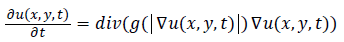
Noise removal: To get rid of noise and unnecessary information, the anisotropic diffusion filter as proposed in [23] is utilized. This filter removes the noise from input image while preserves important parts of image contents such as edges and major boundaries. The filtered image is modeled as the solution to the anisotropic diffusion equation as follows:
 (1)
(1)
where  is a scale image and
 is a decreasing function depending on the gradient of u .
Edge and boundary extraction: An edge gives us an object layout. Identifying the pixel value and it is compared with the neighboring pixels to be outlined as edge regions [24]. All objects in the image are outlined when the intensities are measured exactly [25]. In order to extract the edges and boundaries from images, canny edge detection algorithms [24] is utilized. In Canny edge detection procedure for segmentation shows in Figure 4.

Figure 4. OPG image for After Edge and Boundary Detection.
Feature extraction
Mostly, image classification use low level features color, shape and texture. But, DR images are mainly in grey level. So, color is not suitable feature for DR analysis. Then, shape and texture can be considered for DR analysis [12]. Here, we extracted the conventional features in Figure 5 as follows: Shape, Region properties, Tamura features, entropy and Wavelet based Texture Features for two-Dimensional level discrete wavelet transform for four (LL, LH, HL and HH) sub-bands in θ directions(θ=0°, 45°, 90°, 135°). Here, there are 383 features are extracted from each DR image.

Figure 5. Conventional features.
Shape features: Shape provides geometrical information of an object in an image. This geometrical information is remained same even when the location, scale and orientation of the object are changed. In this study, the shape information of an image is described based on its edges. A histogram of the edge directions is used to represent shape attribute for each image and image patches.
Edge direction histogram (EDH): For each pixel its edge vector is
defined as
its edge vector is
defined as  where
where and
and  are obtained by
the vertical edge mask and horizontal edge mask respectively.
The edge vector can be also represented as its amplitude and
direction, the amplitude can be roughly estimated by
are obtained by
the vertical edge mask and horizontal edge mask respectively.
The edge vector can be also represented as its amplitude and
direction, the amplitude can be roughly estimated by
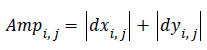 (2)
(2)
The angle representing the pixel’s edge direction is decided by
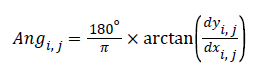 (3)
(3)
Each pixel in the image has an edge vector containing its edge
amplitude and direction, and all the pixels’ edge vectors form
the image’s edge map. It must be noted that in the actual
implementation of the algorithm, equation (3) is not necessary.
In this paper, the  is used to express the pixel’s edge
direction.
is used to express the pixel’s edge
direction.
The edge direction histogram [26] is used to compare the edge information between the distorted image blocks and the reference ones. In this paper, the continual direction (0°~180°) is divided into 8 discrete directions which are shown in Figure 6 and are not the same as reference [26].

Figure 6. The 8 discrete directions.
For each image block, its edge direction histogram can be obtained by the following steps:
Step 1. Calculate each pixel’s edge amplitude and direction by equations (2) and (3) respectively.
Step 2. Quantify each pixel’s direction as one of the 8 discrete directions (see Figure 6).
Step 3. Sum up all the pixels’ edge amplitudes with the same direction in the block.
Now edge direction histogram (vector) is obtained. An example of a 16 × 16 image block and its edge direction histogram are showed in Figure 7.

Figure 7. A 16 × 16 image block and its edge direction histogram, D represents the directions and AMP represents the amplitude.
Wavelet-texture features: Various statistical features are derived from the segmented image for classification [17]. But it is a challenging task to extract a good feature set for classification. GLCM features are based on the joint probability distribution of matchup of pixels. Distanced and angle ө within a given neighborhood are used for computation of joint probability distribution between pixels. Normally d=1, 2 and ө=0°, 45°, 90°, 135° are used for computation [27]. Hence, 32 features totally obtained each DR image. In our proposed system the following GLCM features are extracted [28]:
Energy (k1) which expresses the repetition of pixel pairs of an image,
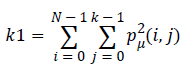 (4)
(4)
Local variations (k2) which present in the image is calculated by Contrast. If the contract value is high, the image has large variations.
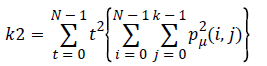 (5)
(5)
Correlation (k3) is a measure linear dependency of grey level values in co-occurrence matrices. It is a two dimensional frequency histogram in which individual pixel pairs are assigned to each other on the basis of a specific, predefined displacement vector.
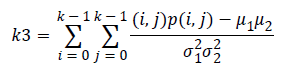 (6)
(6)
Homogeneity (k4) is inversely proportional to contrast at constant energy whereas it is inversely proportional to energy.
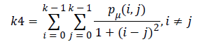 (7)
(7)
Wavelet transform can capture both frequency and spatial information and has merits of multi-resolution and multi-scale decomposition [29,30]. The selection of the wavelet base is very important in practical applications of DWT. When analyzing the same problem, a different wavelet basis will produce a different result. So far, there has been no good way or a unified standard to solve the problem, and the main method used is to determine a wavelet base that is applicable for a problem according to the error between the results derived from wavelet analysis and the theoretical results.
In our study, we selected the well-known Zero tree Wavelet as the wavelet base, which may provide a more effective analysis than others in the scenario of image processing. In order to perform the DWT, the image has to be a square image, and its row/column size must be an integer power of 2. So, technically, the EZW is applicable to the square images of sizes in integer powers of 2 (for example, image sizes like 128 x 128 or 512 x 512). This transformation is theoretically lossless, although this may not always be the case. The purpose of the transformation is to generate decorrelated coefficients, which means it removes all the dependencies between samples.
The EZW algorithm applies Successive Approximation Quantization in order to provide multi-precision representation of the transformed coefficients and to facilitate the embedded coding. The algorithm codes the transformed coefficients in decreasing order in several scans. Each scan of the algorithm consists of two passes: significant map encoding and refinement pass. The dominant pass scans the subband structure in zigzag, right-to-left and then top-to-bottom within each scale, before proceeding to the next higher scale of subband structure as presented in Figure 8.

Figure 8. EZW subband structure scanning order.
After decomposition for the first time, the original image is divided into four sub-band images of equal size of that quarter. These four images are LLi, LHi, HLi and HHi, which represent the ith scale. The sub-band LLi represents the low-frequency sub-image, corresponding to an approximation image, which is to be decomposed in the (i+1)th scale; the sub-bands LHi, HLi and HHi collectively called low-frequency sub-images correspond to detail images. In first-level decomposition, the size of the original image of size M×N is decomposed into four sub-bands LL1, LH1, HL1 and HH1, of size M/2×N/2. After the ith-level decomposition, the size of the three sub-bands LHi, HLi and HHi is M/2i×N/2i [31].
Region properties: The common region properties [32] are perimeter, eccentricity, Euler number, area, major axis length, minor axis length and orientation of the image. The minor and major axis lengths are lengths of the minor and major axes of the ellipse that has the same normalized second central moments as the region or an object respectively. The eccentricity can be defined as the ratio of the smallest eigenvalue to the largest one. The Euler number is the subtraction of number of connected components and number of holes in the object or region. The orientation can be defined as the direction of the largest eignvector of the second order covariance matrix of a region or an object. The perimeter is the number of pixels located on the object boundary and the area is the number of pixels located in the region within the boundary.
Tamura features: There are 6 different Tamura features: coarseness, contrast, directionality, linelikeness, regularity and roughness [33]. In the literature [34], the first three features are used since they are strongly correlated with human perception.
Entropy: It is a general statistical parameter. Log-Energy entropy, Sure entropy and Shanon entropy [35], shown in Equation (8), are generally used to extract feature [36].
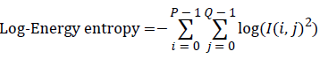
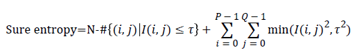
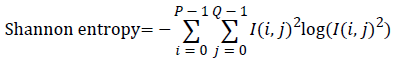 (8)
(8)
Where  and
and 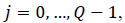 is the
image with size
is the
image with size  is a constant where
  N is the
total number of pixels in image I and “#” denotes the number of
elements in the set. As the information theoretical features like
Entropy, depend on gray level intensities, the images gray level
should be normalized before feature extraction until exact and
accurate features are generated. Hence, to normalize the gray
level intensities, Equation (9) is utilized. If
N is the
total number of pixels in image I and “#” denotes the number of
elements in the set. As the information theoretical features like
Entropy, depend on gray level intensities, the images gray level
should be normalized before feature extraction until exact and
accurate features are generated. Hence, to normalize the gray
level intensities, Equation (9) is utilized. If  is the original
image pixel, the normalization equation is:
is the original
image pixel, the normalization equation is:
 (9)
(9)
Where  and
and  are the initial (desired) mean and variance of
original image I, respectively and
are the initial (desired) mean and variance of
original image I, respectively and  is the normalized image.
In this paper, the desired mean and variance are selected 100
and 2000 respectively. After the normalization, three different
types of Entropy features are extracted which provide a three
element feature vector.
is the normalized image.
In this paper, the desired mean and variance are selected 100
and 2000 respectively. After the normalization, three different
types of Entropy features are extracted which provide a three
element feature vector.
Feature selection
Feature selection [18] retains higher accuracy at the use of minimal feature subset. It can be accomplished through wrapper and filter methods. Wrappers depend heavily on classification algorithm to measure the prominence of a feature to be included in the model. Feature selection through wrappers generally performs better than filters because the filter selection is optimized for the particular learning algorithm to be used. Wrapper methods are very time taking and they are computationally expensive. Here, Random Forest (RF) algorithm is used as a feature selection method [18].
Random forest (RF): It is the most popular machine learning method, but it also provides feature importance for their relatively good accuracy, robustness and ease of use [37]. It consists of a number of decision trees. Building many decision tree predictors with randomly selected variable subsets and utilizing a different subset of training and validation data for each individual model. After generating many trees, aggregate voting of all trees in the forest based class prediction occurred. Thus, lower ranked variables are eliminated based on empirical performance heuristics [18]. The main advantages of RF are: handles numerous inputs attributes - both qualitative and quantitative, estimate relatively important features for feature selection, fast learning and modest computation time. In Table 2, shown the Number of features selected based on the feature selection methods.
| Feature Selection Methods | Number of Features Selected |
|---|---|
| Before Feature Selection | 383 |
| PCA | 41 |
| PSO | 45 |
| RF | 35 |
Table 2. Summary of Feature Selection.
Classification
In mid-1990s, Vapnik [38] introduced Support Vector Machine (SVM). It performs well in small sample sizes and in high dimensional spaces [19]. It also exploits the least feasible quadratic programming issues, which determines systematically and promptly. It improves the scaling and computing time significantly. It executes the lowest sequential maximization procedure to train a classifier using linear kernels.
Support Vector Machine (SVM) is a kernel based technique that represents one of the major developments in machine learning algorithm. SVM is a group of supervised learning methods that can be applied for classification and regression. It learns by example to assign labels to objects. SVM has shown its capacities in pattern recognition and a better performance in many domains compared with other machine learning techniques. SVMs have also been successfully applied to an increasingly wide variety of biological applications. Based on empirical results and several classification applications in automatic classification of medical X-ray images, SVM has shown a better generalization performance compared with other classification techniques [40-42].
SVM algorithm takes a set of input data points. It then decides that the data point belong to which possible two classes. The aim is to construct a hyperplane or set of hyperplanes in a high or infinite dimensional space that classifies the data more accurately. Therefore, the basic idea is to find a hyperplane that has the greatest distance to the nearest training data points of any class.
A hyperplane can be defined by the following equation:
wx +b=0 (10)
Where x is the data point lying in the hyperplane, w is normal vector to hyperplane and b is the bias. Figure 9 and 10 show the basics of SVM.

Figure 9. The basics of classification by SVM.

Figure 10. Proposed Model for RF-SVM.
The idea is to separate two classes (red circle and blue circle), each are labeled as 1 and -1 respectively. Those circles which lie on p1 and p2 are support vectors. For all data points from the hyperplane p (wx + b = 0), the distance between origin and the hyperplane p is (|b|||w||). We consider the patterns from the class -1 that satisfy the equality wx + b = -1, and determine the hyperplane p1; the distance between origin and the hyperplane p1 is equal to ||-1-b|||w||.
Similarly, the patterns from the class +1 satisfy the equality wx + b = +1, and determine the hyperplane p2; the distance between origin and the hyperplane p2 is equal to |+1−b|||w||. Of course, hyperplanes P, P1, and P2 are parallel and no training patterns are 44 located between hyperplanes P1 and P2. Based on the above considerations, the margin between hyperplanes P1 and P2 is 2||w||.
In order to use the SVM methodology to handle the classes
are not linearly separable, then the input vectors such as low
level feature vectors are mapped to higher dimensional feature
space H via a nonlinear transformation, Rd→ H. The kernel
function (K(xi,xj)) is used then to construct optimal hyperplane in
this high dimensional feature space. This kernel function is a
products of input vector  Radial Basis Function (RBF) kernel and Polynomials kernel are
the most common mappings:
Radial Basis Function (RBF) kernel and Polynomials kernel are
the most common mappings:
Polynomials kernel: K xi,xj=(xi.xj+1)q. (q is the degree of Polynomial)
Radial Basis Function (RBF) kernel:  (σ is the Gussian sigma)
The above description of SVM is designed for binary classification which only deals with two class labels +1 and -1. It can be extended to multi-class classification where each data point x can be mapped to a specific label y from the set of available labels.
In our proposed system the classification has two divisions: i) training stage and ii) testing stage. In the training stage, various features are extracted from the IAN identified and not identified images. In testing stage based on the knowledge base, the classifier classifies the image into IAN- identified and not identified images. Figure 10 shows the Proposed RF-SVM model for feature selection based classification model.
Experimental Results and Discussions
Data description
Here, 140 OPG DRs collected from MSR Tooth Clinic, Madurai which is composed of 62 OPG radiographs for male patients of age of 10 to 75 years old and 38 for female patients of age of 12 to 74 years old. Around 40 OPG radiographs are posterior dental implants for accuracy of implant position and injuries of IAN. The diagnostic decisions of all the 100 patients were made by a radiologist panel. Table 3 show the summary of experimental data of OPG image and Patients Data Summary with Sex and Age Range in Table 4.
| Patient Age (Years) | Sex | Number of Patients | Number of DRs | Data Dimensions |
|---|---|---|---|---|
| 10-75 | Male-62 | 100 | 140 | 1024 × 564 × 24 |
| Female-38 |
Table 3. Summary of Experimental Data.
| Age Range | Male | Female | Total |
|---|---|---|---|
| 10 to 20 | 15 | 8 | 23 |
| 21 to 35 | 27 | 20 | 47 |
| 36 to 50 | 22 | 17 | 39 |
| 51 to 65 | 10 | 8 | 18 |
| 66 to 75 | 9 | 4 | 13 |
| Total | 83 | 57 | 140 |
Table 4. Patients Data Summary with Sex and Age Range.
Performance assessment
In this study, classification accuracy, sensitivity and specification were used as assessment of the proposed RFSVM model. It defined in Equation (11), (12) and (13).
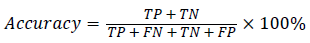 (11)
(11)
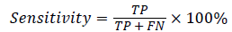 (12)
(12)
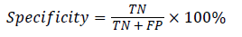 (13)
(13)
where TP(True Positive) denote the number of correctly classified IAN injured object, TN(True Negative) denote the number of correctly classified healthy object, FP(False Positive) denote the number of normal cases incorrectly classified. IAN denotes injured object and FN (False Negative) denotes the number of irregular objects incorrectly classified as normal object.
Comparison of classification performance
The obtained experimental results from the proposed technique are given in Table 5 and Table 6. The accuracy of SVM classification accuracy is better than Decision Tree (DT) and Multilayer Perceptron (MLP) classifiers. Both training and testing stages of Random Forest (RF) - Support Vector Machine (SVM) get better classification accuracy of 96.4% and 83.58% respectively. The graphical result Figures 11 and 12 showed the comparison of proposed results with existing Results [13,14,39].
| Feature Selection + Classifier |
Classification Accuracy | Sensitivity | Specificity |
|---|---|---|---|
| PCA - DT [13] | 82.3 | 76.2 | 85.2 |
| PCA - MLP [14] | 85.4 | 76.6 | 90.2 |
| PSO - MLP [39] | 88.7 | 85.2 | 88.5 |
| RF - SVM (Proposed) | 96.4 | 88.2 | 99.1 |
Table 5. Comparison of Training results with Different classifiers.
| Feature Selection + Classifier |
Classification Accuracy | Sensitivity | Specificity |
|---|---|---|---|
| PCA - DT [13] | 78.58 | 68.6 | 76.8 |
| PCA - MLP [14] | 79.29 | 69.9 | 83.8 |
| PSO - MLP [39] | 80.71 | 77.6 | 80.5 |
| RF - SVM (Proposed) | 83.58 | 79.9 | 92.8 |
Table 6. Comparison of Testing results with Different classifiers.

Figure 11. Performance analysis for classification accuracy.

Figure 12. Performance analysis for Sensitivity and Specificity for training and classification stage.
In the proposed system, experimental results are compared to medical expert results with proposed system results in Table 7.
| IAN Identification | Medical Experts | PCA-DT | PCA-MLP | PSO-MLP | RF-SVM | |||||
|---|---|---|---|---|---|---|---|---|---|---|
| No. of Images | % | No. of Images | % | No. of Images | % | No. of Images | % | No. of Images | % | |
| Not Identified | 12 | 8.57 | 8 | 5.71 | 7 | 5 | 7 | 5 | 5 | 3.57 |
| Partially Identified | 25 | 17.86 | 22 | 15.71 | 22 | 15.71 | 20 | 14.29 | 18 | 12.86 |
| Clearly identified | 103 | 73.57 | 110 | 78.58 | 111 | 79.29 | 113 | 80.71 | 117 | 83.58 |
Table 7. Comparison of Different Classifier Results with Medical Experts.
Above the experimental data in table 7, we got the following results.
Not identified in IAN from medical experts 8.57%, but the proposed system has 3.57% only.
Partially identified in IAN, 17.86% for medical experts and 12.86% for the proposed system.
Clearly identified in IAN, 73.57% for medical experts, 83.58% for proposed system.
The total number of partial and clearly identified IAN is 91.43% for medical experts and 96.44% for proposed system. Comparatively, the proposed system clearly identified IAN is 5% more than medical experts. So, the proposed system has improved accuracy of IAN identification then medical experts. Figure 13 shows the graphical representation of medical expert results with proposed system results.

Figure 13. Comparison of IAN Identification.
In Tables 8-12 to be discussed in the age range classification of IAN identification with medical experts, PCA-DT, PCAMLP, PSO-MLP and RF-SVM respectively. Below the age of 15 and more than age of 65, the visibility of IAN is very limited.
| Age Range | Not Identified | Partially Identified | Clearly identified | |||
|---|---|---|---|---|---|---|
| Male | Female | Male | Female | Male | Female | |
| 10 to 20 | 4 | 2 | 7 | 5 | 4 | 1 |
| 21 to 35 | 0 | 0 | 2 | 1 | 25 | 19 |
| 36 to 50 | 0 | 0 | 1 | 0 | 21 | 17 |
| 51 to 65 | 1 | 0 | 1 | 2 | 8 | 6 |
| 66 to 75 | 3 | 2 | 5 | 1 | 1 | 1 |
| Total | 8 | 4 | 16 | 9 | 59 | 44 |
Table 8. Summary of IAN identification for medical experts.
| Age Range | Not Identified | Partially Identified | Clearly identified | |||
|---|---|---|---|---|---|---|
| Male | Female | Male | Female | Male | Female | |
| 10 to 20 | 3 | 1 | 6 | 5 | 6 | 2 |
| 21 to 35 | 0 | 0 | 2 | 0 | 25 | 20 |
| 36 to 50 | 0 | 0 | 1 | 0 | 21 | 17 |
| 51 to 65 | 0 | 0 | 1 | 1 | 9 | 7 |
| 66 to 75 | 2 | 2 | 5 | 1 | 2 | 1 |
| Total | 5 | 3 | 15 | 7 | 63 | 47 |
Table 9. Summary of IAN Identification for PCA-DT Classifier.
| Age Range | Not Identified | Partially Identified | Clearly identified | |||
|---|---|---|---|---|---|---|
| Male | Female | Male | Female | Male | Female | |
| 10 to 20 | 2 | 1 | 6 | 4 | 7 | 3 |
| 21 to 35 | 0 | 0 | 0 | 1 | 27 | 19 |
| 36 to 50 | 0 | 0 | 1 | 0 | 21 | 17 |
| 51 to 65 | 0 | 0 | 1 | 2 | 9 | 6 |
| 66 to 75 | 2 | 2 | 5 | 2 | 1 | 1 |
| Total | 4 | 3 | 13 | 9 | 65 | 46 |
Table 10. Summary of IAN Identification for PCA-MLP Classifier.
| Age Range | Not Identified | Partially Identified | Clearly identified | |||
|---|---|---|---|---|---|---|
| Male | Female | Male | Female | Male | Female | |
| 10 to 20 | 2 | 1 | 5 | 4 | 8 | 3 |
| 21 to 35 | 0 | 0 | 1 | 0 | 26 | 20 |
| 36 to 50 | 0 | 0 | 1 | 0 | 21 | 17 |
| 51 to 65 | 0 | 0 | 1 | 1 | 9 | 7 |
| 66 to 75 | 3 | 1 | 6 | 1 | 1 | 1 |
| Total | 5 | 2 | 14 | 6 | 65 | 48 |
Table 11. Summary of IAN Identification for PSO-MLP Classifier.
| Age Range | Not Identified | Partially Identified | Clearly identified | |||
|---|---|---|---|---|---|---|
| Male | Female | Male | Female | Male | Female | |
| 10 to 20 | 2 | 1 | 10 | 3 | 3 | 4 |
| 21 to 35 | 0 | 0 | 0 | 0 | 27 | 20 |
| 36 to 50 | 0 | 0 | 0 | 0 | 22 | 17 |
| 51 to 65 | 0 | 0 | 1 | 0 | 9 | 8 |
| 66 to 75 | 1 | 1 | 2 | 2 | 6 | 1 |
| Total | 3 | 2 | 13 | 5 | 67 | 50 |
Table 12. Summary of IAN Identification for RF-SVM Classifier.
Conclusion
In this paper, unified RF-SVM model based on EZW based texture and shape features are proposed. It was performed on a database consisting 140 DRs. By the aim of improving the classification accuracy, different conventional features are extracted. Then, Random Forest based Support Vector Machine model was used for feature selection and classification process. Experimental results shows that our method is an effective feature selection method obtain higher classification accuracy of other methods. Other performance analysis like sensitivity and specificity of our proposed model perform get better than other methods. The provided results show effectively classifies the IANI identification.
References
- Mischkowski RA, Zinser MJ, Neugebauer J, Kubler AC, Zoller JE. Comparison of static and dynamic computer-assisted guidance methods in implantology. Int J Computerized Dentistry 2006; 9: 23-35.
- Mansoor J. Pre-and postoperative management techniques. Before and after. Part 1: medical morbidities. British dental journal 2015; 218; 273-278.
- Modi CK, Desai NP. A simple and novel algorithm for automatic selection of ROI for dental radiograph segmentation. in Proc. 24th IEEE CCECE 2011; 504-507.
- Haring JI, Jansen L. Dental radiography: principles and techniques. London: W. B. Saunders Company 2000; 342-362.
- White SC, Pharoah MJ. Oral radiology: principles and interpretation. Elsevier Health Sciences 2014.
- Iwao S, Ryuji U, Taisuke K, Takashi Y. Rare courses of the mandibular canal in the molar regions of the human mandible: A cadaveric study. Okajimas folia anatomica Japonica 2014; 82: 95-102.
- Malik NA. Textbook of Oral and Maxillofacial Surgery. 2nd ed, New Delhi: Jaypee Brothers Medical Publishers 2008.
- Kim HG, Lee JH. Analysis and evaluation of relative positions of mandibular third molar and mandibular canal impacts. Journal of the Korean Association of Oral MaxillofacSurg 2014; 40: 278-284.
- Kim JW, Cha IH, Kim SJ, Kim MR. Which risk factors are associated with neurosensory deficits of inferior alveolar nerve after mandibular third molar extraction. J Oral MaxillofacSurg 2012; 70: 2508-2514.
- Karthikeyan T, Manikandaprabhu P. Analyzing Urban Area Land Coverage Using Image Classification Algorithms. Computational Intelligence in Data Mining-Volume 2, Smart Innovation, Systems and Technologies, Springer India 2015; 32: 439-447.
- Yu P, Xu H, Zhu Y, Yang C, Sun X, Zhao J. An automatic computer-aided detection scheme for pneumoconiosis on digital chest radiographs. J Digit Imaging 2011; 24: 382-393.
- Katsuragawa S, Doi K, MacMahon H, Monnier-Cholley , Morishita J, Ishida T. Quantitative analysis of geometric-pattern features of interstitial infiltrates in digital chest radiographs: preliminary results. J Digit Imaging 1996; 9: 137-144.
- Karthikeyan T, Manikandaprabhu P. A Novel Approach for Inferior Alveolar Nerve (IAN) Injury Identification using Panoramic Radiographic Image. Biomed Pharma Jour 2015; 8: 307-314.
- Karthikeyan T, Manikandaprabhu P. A Study on Digital Radiographic Image Classification for Inferior Alveolar Nerve Injury(IAN) Identification using Embedded Zero Tree Wavelet. International Journal of Applied Engineering Research 2015; 10: 599-604.
- Mueen A, Zainuddin R, Sapiyan Baba M. Automatic Multilevel Medical Image Annotation and retrieval. J Digit Imaging 2008; 21: 290-295.
- Tommasi T, Orabona F, Caputo B. Discriminative cue integration for medical image annotation. Pattern Recogn Lett 2008; 29: 1996-2002.
- Haralick RM, Shanmugam K, Dinstein I. Textural features for image classification. IEEE Trans Syst Man Cybern 1973; 3: 610-621.
- Han L, Embrechts M, Szymanski B, Sternickel K, Ross A. Random forests feature selection with K-PLS: detecting ischemia from magnetocardiograms. in Proc. ESANN, Bruges, Belgium 2006; 221-226.
- Zhu Y, Tan Y, Hua Y, Wang MP, Zhang G, Zhang JG. Feature selection and performance evaluation of support vector machine (SVM)-based classifier for differentiation benign and malignant pulmonary nodules by computed tomography. J Digit Imaging 2010; 23: 51-65.
- Yuan QF. Cancer Diagnosis by Using Support Vector Machine. MD dissertation, Chongqing University 2007.
- Lu Y. Automatic topic identification of health-related messages in online health community using text classification Springer plus 2013; 309.
- Ghofrani F, Helfroush M, Danyali H, Karimi K. Medical X-ray image classification using gabor-based CS local binary patterns. in Proc. ICEBEA 2012.
- Fu S, Ruan Q, Wang W, Li Y. Adaptive anisotropic diffusion for ultrasonic image denoising and edge enhancement. Int J Info Tech 2006; 2: 284-292.
- Canny J. A computational approach to edge detection. IEEE Trans Pat Anal Mach. Intell 1986; 8: 679-698.
- Jian M, Liu L, Guo F. Texture image classification using perceptual texture features and Gabor wavelet features. in Proc APCIP 2009.
- Feng P, Xiao L, Rahardja S. Fast mode decision algorithm for intraprediction in H.264/AVC video coding. IEEE Trans. Circuits and Syst. Video Tech 2005; 813- 822.
- Gelzinisa A, Verikasa A, Bacauskienea M. Increasing the discrimination power of the co-occurrence matrix-based features. Pattern Recogn 2004; 40: 2367-2372.
- Subramoniam M, Barani S, Rajini V. A non-invasive computer aided diagnosis of osteoarthritis from digital x-ray images. Biomedical Research 2015; 26: 721-729.
- Arivazhagan S, Ganesan L. Texture segmentation using wavelet transform. Pattern Recogn Lett 2003; 24: 3197-3203.
- Kociołek M, Materka A, Strzelecki M, Szczypiński P. Discrete Wavelet Transform –Derived Features for Digital Image Texture Analysis”. in Proc. Int. Conf. Signals and Electronic Systems. Lodz, Poland: IEEE 2001.
- Wu PC, Chen LG. An efficient architecture for two-dimensional discrete wavelet transform. IEEE Trans. Circuits and Syst Video Tech 2001; 11: 536-545.
- Masood K, Rajpoot N. Spatial analysis for colon biopsy classification from hyperspectral imagery. Annuals of the BMVA 2008; 2008: 1-6.
- Muller H, Cramer JK, Eggel I, Bedrick S, Reisetter J, Kahn CE Jr, Hersh W. Overview of the CLEF 2010 medical image retrieval track. in Proc CLEF 2010 Workshop 2010.
- Prasad BG, Krishna AN. Performance evaluation of statistical textural features for medical image classification. in Proc National Conference on Emerging Trends in Computer Science 2011.
- Coifman RR, Wickerhauser MV. Entropy-based algorithms for best basis selection. IEEE Trans Information Theory 1992; 38: 713-718.
- Vasantha M, Bharathi DVS, Dhamodharan R. Medical image feature, extraction, selection and classification. Int J Engg Sci & Tech 2010; 2: 2071-2076.
- Breiman L. Random forests. Machine Learning 2001; 45: 5-32.
- Vapnik VN, Vapnik V. Statistical Learning Theory. Newyork: Wiley 1998.
- Karthikeyan T, Manikandaprabhu P. Feature Selection Based Hybrid Classification Algorithm with Embedded Zero Tree Wavelet. ARPN J Engg Appl Sci 2015; 10: 1723-1731.
- Mueen A, Zainuddin R, Sapiyan Baba M. Automatic multilevel medical image annotation and retrieval. J Digit Imaging 2008; 21: 290-295.
- Rahman MM, Desai BC, Bhattacharya P. Medical image retrieval with probabilistic multi-class support vector machine classifiers and adaptive similarity fusion. Comput Med Imaging Graph 2007; 32: 95-108.
- Unay D, Soldea O, Ozogur-Akyuz S, Cetin M, Ercil A. Medical image retrieval and automatic annotation: VPA-SABANCI at ImageCLEF 2009. in Proc Cross-Language Evaluation Forum (CLEF) Workshop in conjunction with ECDL’09 Corfu Greece 2009.