ISSN: 0970-938X (Print) | 0976-1683 (Electronic)
Biomedical Research
An International Journal of Medical Sciences
Research Article - Biomedical Research (2016) Computational Life Sciences and Smarter Technological Advancement
Time series analysis and identification of rsn using GLM-ICA two class classifier
Department of ECE, College of Engineering, Guindy, Anna University, Chennai, India
- *Corresponding Author:
- SP Thaiyalnayaki
Department of ECE, College of Engineering
Anna University, India
Accepted date: April 15, 2016
The functionally receptive regions of the brain had always been concealing themselves even from the functional MRIs. This induced the quest of finding an efficient algorithm to address the issue of functional localization of activated regions and classification of the active functional areas of the brain. A sample of 10 Healthy controls and 3 shaky hand septuagenarians, nine acquisitions was considered for this study. The fMRI of three motor imbalance subjects whose scan size was 128 × 128 × 23 and a total of 110 volumes accompanied by three acquisitions for each, who are on an average of 65 ± 3 years were subjected to examination. The conclusion derived from this commendable study was that the number of voxels awakened in the sensory motor network was more in tremulous subjects. Besides the activation of the sensory motor network, tightly localized spatial variations were observed in default mode network (DMN), auditory network, sensory motor and visual networks (medial, occipital), right and left executive control networks of these people. This lead to GLM-ICA two class classifier for decision support which performs pre-processing each rsfMRI scan, encompassing realignment, coregistration, normalisation and smoothing, Extracting independent components from smoothed output, Selecting highest Eigen vectors for retrenching the high-dimensionality of the gathered neuroimages time series, Evolving 2-class classifier using k-means algorithm. The proposed algorithm GLM-ICA two class classifier aided the classification of about 87.5% of the functional localization.
Keywords
Terms-Rest fMRI, Sensory motor network, Independent component analysis, PCA, K-means clustering.
Introduction
The objective of fMRI analysis is to assess the activity of each voxel upon activation. fMRI data typically consist of individual time series associated with the voxels of the brain. The significance of the response of each individual voxel to the stimulus is assessed by statistically analysing the associated fMRI time series. Statistical analysis of image data relates to data modelling, to get observed responses as components of interest and error, making surmising about fascinating impacts using the variances of the partitions and then testing for significance. Hypothesis-driven methods, similar to standard GLM, endeavour to fit information to hypotheses [1]. However, the limitation of hypothesis-driven univariate methods is that they rely on the prior information of hemodynamic response and are unable to examine interactive and coordinated responses from multiple brain regions. A strategy for analysing fMRI data based on ICA was adapted which allows the extraction of both transient, task-related, non task-related and various artifactual components of the observed fMRI signals [2]. In addition, it has been reported that lowfrequency oscillations are in the range of 0.1 Hz or lower contributed most to the temporal structure of the auditory, visual and sensory motor functional connectivity maps [3,4]. Also Spatial Independent Component Analysis of fMRI gives an extremely high degree of consistency in spatial, temporal, and frequency parameters within and between subjects [5]. A method of constrained ICA by imposing regularization on certain estimated time courses using the paradigm information, is used to effectively extract the target components. The prior information constrains one or more specific components to be close to a paradigm-derived time course and improves the robustness of ICA in the presence of noise [6].
Considering that the components for each voxel are sparse and the neural integration of the dynamics is linear, the sparse dictionary learning algorithm [7-9] is utilized to identify each component. The sparsity of underlying hemodynamic signals take interactions between voxels and characterize brain responses as spatial-temporal patterns. This highlight the activated voxels considered for the analysis. Three types of estimation can be obtained, Fully Bayesian, when the priors are known, Empirical Bayesian, when the priors are obscure yet they can be parameterized and maximum likelihood estimation, when the priors are assumed to be flat. All these procedures can be implemented with an EM algorithm [10]. To localize the spatial map and time courses, three fMRI task datasets, ten Healthy subject’s rest data and three Shaky hand subjects rest data, 9 volumes were employed for comparisons. Strategies considered for quantifying the performance of the algorithms were the correlation analysis and Number of voxels. To evaluate the respective accuracies on estimated time courses and spatial layouts from the Rest and the fMRI task dataset, the demonstration is performed using MATLAB and various other toolboxes, SPM, Marsbar and ICA. The remaining parts of the paper were organized as follows. The theory of the post processing techniques by statistical analysis using GLM, followed by ICA and 2-class classification is described in section II. Section III provides experimental results while Section IV gives the Discussion and Conclusion
Theory
Statistical parametric mapping (SPM)
An fMRI time series y of block observations can in general be modeled as the general linear equation,
y=xβ+Є→(1)
Where y in (1) is a vector of measured data, ϵ is error term measures the difference between the data y and xβ and x is design matrix. In GLM model the data can remove drift and respiration if they can be modeled. The β terms are the parameters that define the contribution of each component of the design matrix to the value y, estimated so as to minimize the error β is a matrix containing parameters which are estimated using ordinary least square equation as in Equation (2). Changes in blood oxygenation are statistically modeled using GLM, the inferences are made about task specific changes in neuron activation.
β̂=(XTX)-1XTY→(2)
The fMRI dataset has to be preprocessed before performing statistical analysis. On the preprocessed data, in order to ensure the existence of difference between the signal measured in a particular voxel during rest period and task, the significance of parameter estimates are calculated using t-statistics as shown in Equation (3).
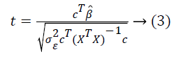
Here c is the contrast value, σ is variance, cT is the transposed contrast vector. To compare experimental conditions, T- or Fstatistics allow testing for a linear combination of β-values that correspond to null hypotheses [4]. Gaussian random field theory (RFT) [5,10] is used to account the spatial smoothness of the statistical map. The SPM12 package is utilized for the analysis of brain imaging data sequences.
Independent component analysis (ICA)
ICA, a multivariate data-driven method has become popular as mentioned in studies [6,7], consider each voxel as a mixture of spatially statistically independent components(ICs). Spatially scattered brain networks, occupied with cognitive process without a priori information, are recognized. Utilizing ICA, spatial patterns and relating time courses are obtained and can think and compare the intelligence of activation in disseminated voxels. Classification of components is not possible with this multivariate method.
fMRI is a widely used brain imaging technique based on the hemodynamic response resulting from neuronal action. Since the hemodynamic response and its connection to neuronal activity are not fully understood, ICA has become a useful approach for identifying either spatially Independent Components (sICA) or temporally Independent Components (tICA) from fMRI data. In general, the ICA decomposition can be represented by the Equation (4)
X=AS→(4)
Where X, is the matrix of observations. A is mixing matrix which contains co-efficient that mixes the independent components in unknown process. S is a matrix which contains desired IC. Both A and S are unknown. In order to find A and S, ICA model assumes the ICs are statistically independent and they have non-Gaussian distributions. Under these assumptions, after estimating the matrix A, its inverse is computed and ICs are obtained from the Equation (5)
S=A-1X→(5)
To estimate A, maximum likelihood estimation or minimization of mutual information can be used. Once ICA has been performed, ICs and their mixing matrix are obtained. The component processes can be represented by differentially activated sparse spatially independent maps. The sum of their activations equals the observed data. An unmixing matrix W can be found by using a statistical method based on the infomax principle [2,6]. In information theory, the probability of a message and its informational content are inversely related, where the mean uncertainty or entropy associated with a set of messages in discrete form is represented by the Equation (6)
H(X) = -ΣKρK logρK→(6)
Where ρk is the probability of the kth event. The joint entropy of two variables is defined by H(X,Y) = H(X) + H(Y) - I(X,Y), where I(X,Y) = H(X) - H(X|Y) is the mutual information, interpreted as the redundancy between X and Y. ICA maximizes the joint entropy of suitably transformed component maps, thus reducing the redundancy between the distributions of map values for different components, resulting in blind separation of the recorded fMRI signals into spatially independent components [2]. W is initialized to identity matrix and H(y) is maximized iteratively, where y=g(C), C=WXs, and g(C) is predefined nonlinear function. Here, Xs is a data matrix defined by

where
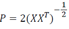
(XXT) is the N × N covariance matrix of the data X. The nonlinear function g(C), which provides necessary higher-order statistical information, is chosen to be the logistic function
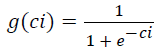
This directs the algorithm towards finding component maps with relatively few highly active voxels. The elements of W, are updated using data vectors drawn randomly from {Xs} without substitution, according to
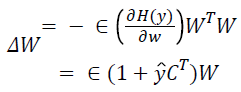
Where Є a learning rate (typically near to 0.01) and the vector ŷ has elements
ŷ = (1-2y)
During training, the learning rate is reduced gradually until the weight matrix W stops changing appreciably. A principal advantage of ICA is its appropriateness to standards in which prior knowledge of brain responses are not known. However, ICA cannot establish the significance of each IC, the ICA model is not a statistical model that supports classical inference. This is because there is no null model to compare it with. From Equation (4) it is understood that there is no observation error in the ICA model. The optimal number of ICs was determined by a dimension estimation using the minimum description length criterion.
The BOLD time-series was arranged as a matrix Y and Independent component maps were obtained for all the acquisitions. Activations that are unanticipated, that is brain activations that are only transiently task related (TTR), were more likely to be uncovered by exploratory analysis such as ICA [6,11,12]. Gaussian kernel, 6 mm FWHM smoothing was performed. Once the components were generated using Informax ICA, the voxel values of the spatial map’s Z scores were found, the threshold value for activated voxels was fixed and the activation map of each component was displayed. These were obtained using MATLAB Group ICA. In contrast to PCA, where extracted components are naturally ordered according to variance, ICA does not provide any intrinsic order of ICs [13].
In existing works, interesting and meaningful components are classified from non-neuronal components, contrary to this work where Neuronal and non-neuronal ICs are considered for the classification. As shown in Figure 1, four levels are constructed for the implementation of the proposed GLM-ICA, 2 class classifier. In first level, the 10 healthy controls volumes and 9 abnormal subject rest fMRI scans are individually preprocessed to obtain normalized, Smoothed analyze format scans. In second level 30 independent components are viewed as 30 spatial maps. The 30 time series of each 19 scan is obtained. As the number of iterations are larger, it was decided to have 30 ICs to get perfect classification. Level 3 provides highest 20 Eigen vectors from the array of time series as cell data and their corresponding Eigen independent components, in level four, 2 class k-means clustering is utilized to design a clinical classifier system.

Figure 1. Proposed GLM-ICA, two class classifier.
Experimental Results
Task fMRI
Three task acquisitions are considered for time series analysis viz, auditory task, sensory motor task, visual task. In auditory task data, 96 scans were used for the analysis except for the first head motion and “dummy” twelve scans. Auditory stimulation was presented binaurally at a rate of 60 per min with bi-syllabic words. Slice dimension of each acquisition has a matrix size 64 × 64 with 64 slices and inplane resolution of 3 mm × 3 mm × 3 mm. Next the task set considered for analysis is left hand press for 12 sec and right hand press for 12 sec with rest in between, a total of 302 volumes. The data set of 36 slices with matrix size 64 × 64, inplane resolution of 3 mm × 3 mm × 3.6 mm is used. The task fMRI data was obtained from an open-dataset. The third task data set, visual stimulation obtained as 126 volumes of 61 slices with matrix size 73 × 61 and inplane resolution of 3 mm × 3 mm × 3 mm is analyzed for activation.
Rest fMRI
The rest fMRI data was provided by National Institute of Mental Health and Neuro Sciences (NIMHANS), Bangalore INDIA. The rest fMRI of three subjects analyzed, had scan size 128 × 128 × 23. A total of 110 volumes for each 3 men, 9 acquisitions, mean age=65 ± 3y, scanned on a 3T MR scanner using a gradient echo-planar sequence of axial slice orientation of 23 slices, TE=40 ms, flipangle=90°, voxelsize=1.8 × 1.8 × 6 mm, TR=2460 ms are analyzed for activated voxel regions.
The rest fMRI data in DICOM format is converted to Analyze 7.5 file format using MRICro and preprocessed in SPM and localized using ICA, sparse K-SVD.
Preprocessing for statistical parametric map
First, slice time correction was performed to make the data in each slice correspond to same point in time. The images were then spatially realigned to correct changes in signal intensity over time, which can arise from within-subject head motion during the scanning session. The images in each session were aligned to the first image of the session. The maps were then spatially normalized to a standard Talairach space and resampled to respective voxels. The image volumes were convolved with Gaussian kernel to suppress noise and effects due to residual differences in functional and gyral anatomy during inter subject averaging. The preprocessed output in analyze format is given as input to ICA for functional localization.
fMRI task activations
The auditory task data is preprocessed and 30 independent components are obtained by retaining 99.4075 % of (non-zero) eigenvalues of principle components for data reduction. The stopping criterion for number of iterations of weight update is decided when wchange<10-06 or after 512 iterations. Auditory task converges for 78 iterations with weight change<0.000001 providing 30 ICs. ICA is applied on task and rest brains. Only 30 components are chosen, as it is not essential to select a large quantity of components, due to high component dimensionality. It can also further reduce the chances of identifying a network due to decrease in spatial pattern and spectral properties. In Figure 2 the spatial map of Independent Component number 13 of auditory task and its corresponding time series show tightly localized activation for auditory network. Left motor and right motor task converges for 76 iterations with weight change<0.000001 providing 3o ICs. In Figure 3, the spatial map of Independent Component 15 showing activation in left motor cortex and right cerebellum functional localisation and its corresponding time series implies the most probable identification of functional motor task.

Figure 2. Time series and spatial maps of independent component 13 of auditory task set of 84 acquisitions.

Figure 3. Time series and spatial map of independent component 15 of left and right motor task for 302 acquisitions of task fmri.
The auditory cortex activation map is more pronounced as in Figure 2, than the left motor and right motor activation and the visual cortex activation in Figure 3 and Figure 4. This perfect localization is due to the proper experimental setup of the auditory task than the visual and motor task. Correlation coefficient, obtained from the time series of mean activated voxels and other less activated voxels explain the validity of activation.

Figure 4. Spatial map and time series of independent component no. 18 of visual cortex task of 126 acquisitions.
Activations of rest fMRI
The rest fMRI spatial maps for the recognized Independent component, Default mode network, include the medial prefrontal cortex, the lateral temporal cortex of the left hemisphere, the medial parietal cortex of the right hemisphere, the lateral parietal cortex of the left hemisphere, as in Figure 5.1 is identified in all Healthy and abnormal subjects [14].

Figure 5.1. Spatial map of Subject 3, default mode network.
A total of 570 independent components (ICs) (19 × 30) were labelled after visual inspection by an expert using one of the three possible categories: neuronal, which are relevant IC’s (n=226), non-neuronal, (n=194) and undefined (n=150). The rest fMRI of subject 2 showing the visual occipital activation and of subject 3 showing the Sensory motor network and auditory regions in Figure 5.2a gives an impression that activation is due to speech and unwanted noise heard during scan, Subject 3, rest activations show many regions as visual occipital network, R Executive control network, auditory network, as in Figure 5.3. This may be due to the subjects’ acquisition of information through eyes, noise observance and low level of anxiety and depression.

Figure 5.2. a) Spatial map of Independent Component 12 of subject 2, visual occipital network; b) and C)The Auditory network, Independent Component number 8 of third subject; d) spatial map of IC18, Sensory motor network.

Figure 5.3. a) and b) Subject 3 R & L executive control network IC8,IC11; c) Spatial map of Independent Component no 15 of subject 3 showing BOLD response in Sensory motor network.
The sensory motor network of subject 3 with shaky hands as against the Healthy Controls (HC) was shown in Figures 5.4a and 5.4b. Rest set fMRI Acquisition of Subject 3 shows varied activation regions due to non-silence observance of the subject. Nine healthy subjects whose mean age were 70 years, were compared with the functional activations of 3 abnormal shaky hand subjects, 9 acquisitions, of mean age 65 years.

Figure 5.4. a) Sensory motor region of Healthy subject; b) Spatial map of Independent Component no.15 of BOLD response in Sensory motor network of subject 3. c) Sagittal, coronal, axial view of sensory motor network of subjects.
For rs fMRI of shaky hand subjects, a group ICA is evaluated for 50 components to get the peak voxel coordinates. Cluster size along with Brodmann area is shown in Table 2.
| Component number and IC spatial map | BA | Cluster size VC | Peak voxel location | ||
|---|---|---|---|---|---|
| X | Y | Z | |||
| 18 Sensory Motor network | 6 | 1379 | 18 | -3 | 17 |
| 6 Auditory network | 22 | 1335 | 51 | 38 | 2 |
| 42 Default mode network | 7 | 1663 | -9 | -58 | 26 |
| 46 Visual network | 17 | 1390 | -27 | -76 | -4 |
| 43 Frontal network | 9 | 2409 | -6 | -40 | 5 |
| 24 Attention network | 8 | 1643 | -42 | -55 | 47 |
Table 2. The talairach table associated with each selected RSN BA=Brodmann Area, VC=No of voxels in each cluster, Peak voxel location=Coordinate in mm of tmax in MNI space.
Region of interest
Region of interest of specific task set provides the total number of voxels activated for the visual task and motor task as in Figures 6a and 6b which can be utilized as a mean time series for classification along with independent component time series.

Figure 6. a) The region of interest of visual task activated data set using MARSBAR in SPM, MATLAB shows activations for 2961 voxels in visual medial network . b) The Region of interest of left motor and right motor task activated data set showing activations for 2306 voxels in left motor cortex and right cerebellum.
Two class classifier
As shown in Table 1, the proposed GLM-ICA Two class classifier using cluster PCA is implemented for 128 × 128 × 23 voxels, 1.8 × 1.8 × 6 mm, 110 scan volumes of 9 abnormal subjects and 64 × 64 × 40, 3.44 × 3.44 × 3 mm, 110 volumes of 10 healthy controls. The sensitivity, specificity and accuracy are calculated using
1 Each scan in acquisition is Realigned, Normalized & spatially smoothed. |
Table 1. Algorithm to obtain GLM-ICA two class classifier.
Sensitivity=TP/TP+FN
Specificity=TN/TN+FP
Accuracy=TP+TN/TP+FP+TN+FN
Where TP is true positive, TN true negative, FP false positive and FN false negative
Eighteen highest Eigen values were chosen considering 66.6% of cumulative variance obtained as optimum number from various trials as shown in Figure 8. The specificity of this classifier is nearly 82.36% for 30 trials, accuracy obtained is 87.5% and precision 78%, accounts to fine tune the number of IC chosen or the number of eigen values chosen for GLM-ICA two- class classifier.

Figure 8. Misclassification of healthy people for different Eigen values.18 Eigen values are chosen as optimum.
Discussion and Conclusion
The first aim of this work is to identify corresponding activations in task data and the expected activation in rest data. Then, explored sensory motor cortex functional connectivity in aged subjects Shaky Hand (SH) patients and Healthy Controls (HCs). The contribution lies in constructing a classifier by kmeans on a 2D feature projection space, with group-wise normalization. The results inferred were compared in Figure 5 and Table 3. The rest data network identification as shown in Figure 5 explicitly explains the activation for shaky hand subject. The sensory motor region activation is high as compared to the Healthy subject activations [15-18]. The proposed algorithm, GLM-ICA two class classifier aided the classification of about 87.5% of the functional localization regions of rest fMRI. Independent components identified from the blind source separation and the Eigen values chosen can be fine-tuned to increase classification accuracy. In reference [19] authors worked on task fMRI and ls-SVM based IC fingerprint classifier. The True positive rate of ls-SVM based classifier on the classification of IC-fingerprints, for non-task related components is 90% and as low as 84% using linear discriminant classifier.
| Actual class | Predicted class | |
| 18 | 6 | |
| 3 | 18 | |
Table 3. Confusion matrix for two class classification.
The large voxel activation identification implies that functional localisation can be utilized for the post diagnostic treatment of old age shaky hands subjects, as these shaking unsteadiness and tremors, may act as symptoms of Dementia, Parkinson and alike. The task activations were identified as tightly localized for all the tasks using all the considered hypothetic and data driven methods. The ROI time series can then be utilized to do the performance measure of comparison for Healthy and abnormal subjects. ROI mean signal intensity of each activated task set can be considered for identifying features, along with different independent component time series as shown in Figure 7a and 7b. For assessing region specific activation, SVM-GLM was used with IC fingerprint [20]. This work, GLM-ICA Two-class classifier is the first of its kind to use the IC timeseries Eigen values for classification. The further extension is to identify ROI features, combine with Eigen values and utilize for training the healthy subjects and testing the abnormality of the individual subjects.

Figure 7. a) Mean signal intensity of 126 volumes of visual stimulus task set activated voxels. b) Presence of low frequency components.
Acknowledgment
The Authors would like to thank Professor. Dr Uma Maheshwara Rao, the head of Anesthesia and Academic Dean in NIMHANS, Dr Sri Ganesh, Associate Professor, Department of Neuroanaesthesia in NIMHANS, Bangalore, Dr Saini, Radiologist, NIMHANS for generously providing the required Data.
References
- Friston KJ, Holmes AP, Worsley KJ, Poline JB, Frith CD, Frackowiak RSJ. Statistical parametric maps in functional imaging: A general linear approach. Human Brain Map 1995; 2: 189-210.
- McKeown MJ, Makeig S, Brown GG, Tzyy-Ping J, Kindermann SS, Bell AJ, Sejnowskil TJ. Analysis of fMRI Data by Blind Separation Into Independent Spatial Components. Hum Brain Mapp 1998; 6: 160-188.
- Jezzard P, Matthews PM, Smith SM. Functional MRI: An Introduction to Methods. Oxford University Press, 2001.
- Cordes D, Haughton VM, Arfanakis K, Carew JD, Turski PA, Moritz CH, Quigley MA, Meyerand ME. Frequencies contributing to functional connectivity in the cerebral cortex in resting-state data. Am J Neuroradiol 2001; 22: 1326-1333.
- van de Ven VG, Formisano E, Prvulovic D, Roeder CH, Linden DEJ. Functional Connectivity as Revealed by Spatial Independent Component Analysis of Fmri Measurements During Rest. Hum Brain Mapp 2004; 22: 165-178.
- Calhoun VD, Adali T, Stevens MC, Heil KA, Pekar JJ. Semi blind ICA of fMRI: A method of utilizing hypothesis derived time courses in a spatial ICA analysis. Neuroimage 2005; 25: 527-538.
- Aharon M, Elad M, Bruckstein A. K-SVD: An algorithm for designing overcomplete dictionaries for sparse representation. IEEE Trans Signal Process 2006; 54: 4311.
- Lindquist MA. The Statistical Analysis of fMRI Data. Statistical Sci 2008; 23: 439-464.
- Lee K, Tak S, Ye JC. A Data-Driven Sparse GLM for fMRI Analysis Using Sparse Dictionary Learning With MDL Criterion. IEEE Transact Med Imag 2011.
- Lee K, Tak S, Ye JC. A Data-Driven Sparse GLM for fMRI Analysis Using Sparse Dictionary Learning With MDL Criterion. IEEE Transact Med Imag 2011.
- Kelly RE. Visual inspection of independent components: Defining a procedure for artifact removal from fMRI data. J Neuroscience Method 2010; 189: 233-245.
- Babaie-Zadeh M. Sparse ICA via cluster-wise PCA. Neurocomputing 2006; 69: 1458-1466.
- De Martino F. Classification of fMRI independent components using IC-fingerprints and support vector machine classifiers. NeuroImage 2007; 34: 177-194.
- Buckner RL, Andrews-Hanna JR, Schacter DL. The Brain’s Default Network Anatomy,Function, andRelevance to Disease. Annal New York Academy Sci 2008; 1124: 1-38.
- Greicius MD, Flores BH, Menon V, Glover GH, Solvason HB, Kenna H, Reiss AL, Schatzberg AF. Resting-state functional connectivity in major depression: abnormally increased contributions from subgenual cingulate cortex and thalamus. Biological Psychiatry 2007; 62: 429-437.
- Demertzi A, Gómez F, Crone JS, Vanhaudenhuyse A, Tshibanda L, Noirhomme Q, Thonnard M, Charland-Verville V, Kirsch M, Laureys S, Soddu A. Multiple fMRI system-level baseline connectivity is disrupted in patients with consciousness alterations. Cortex 2014; 52: 35-46.
- Thaiyalnayaki SP, Uma Maheswari O. MLE-Wald and Sparse Dictionary K-SVD Learning for fMRI Post processing Analysis. Int J Knowledge Eng Res 2013; 2: 183-187.
- Wang Z. A Hybrid SVM-GLM Approach for fMRI Data Analysis. Neuroimage 2009; 46: 608-615.
- Soldati N, Robinson S, Persello C, Jovicich J, Bruzzone L. Automatic classification of brain resting states using fMRI temporal signals. Electronics Lett 2009.
- James GA, Tripathi SP, Kilts CD. Estimating brain network activity through back-projection of ICA components to GLM maps. Neuroscience Lett 2014; 564: 21-26.