ISSN: 0970-938X (Print) | 0976-1683 (Electronic)
Biomedical Research
An International Journal of Medical Sciences
- Biomedical Research (2016) Volume 27, Issue 3
The modelling of time-series and the evaluation of forecasts for the future: the case of the number of persons per physician in turkey between 1928 and 2010
1Department of Biostatistics and Medical Informatics,Faculty of Medicine, Izmir University, Izmir, Turkey
2Department of Statistics, Faculty of Sciences, Ankara University, Ankara, Turkey
3Department of Biostatistics, Faculty of Medicine, Ankara University, Ankara, Turkey
Accepted Date: April 03, 2016
Objectives: Health professionals are very important for improving the health status of the society and maintaining a healthy life. The aim of the present study is to model the number of persons per physician via Box-Jenkins and exponential smoothing methods and trend models, to compare these models, and to make estimations for the future. ARIMA or Box-Jenkins models are the combinations of AR and MA models administered to the series differenced at degree d.
Methods: The research material consists of data regarding the number of persons per physician between 1928 and 2010. The data were obtained from STATISTICAL INDICATORS Journal published by the Turkish Statistical Institute. 1928-2010 the number of persons per physician data ARIMA, exponential smoothing, and then modeled by Moving Average methods for future studies (2020) model performance is evaluated.
Results: The goodness of fit criteria of the relevant models. It is seen that the ARIMA (0,1,0) model has the best values except for Mean Absolute Percentage Error (MAPE) and Mean Absolute Error (MAE), but it is the Holt model which has lower mean error.
Conclusion: All administrative works and functions such as planning, organization, management, and rearrangement of healthcare services should be based on the data/evidence to be provided by this institution. Likewise, the problems and effects of healthcare services should be evaluated based on the data of this institution.
Keywords
Time series, Forecasting consistency, ARIMA models, Exponential smoothing methods, Estimation trend.
Abbreviations
ARIMA: Autoregressive Integrated Moving Average; RMSE: The Square Root of Mean Square Errors; MAPE: Mean Absolute Percentage Error; MAE: Mean Average Error; MaxAPE: Maximum Absolute Percentage Error; MaxAE: Maximum Absolute Error; Norm. BIC: Normalized Bayesyan Information Criterion.
Introduction
Health professionals are very important for improving the health status of the society and maintaining a healthy life. Therefore, the number of employees working in the field of health, their education, the place they receive education, and the units or departments where they provide service are of great importance. Effective and productive healthcare services require sufficient number of health professionals, their training in accordance with contemporary criteria, and their balanced distribution across the country through a good planning.
According to the statistical indicators (1923-2011) data published by the Turkish Statistical Institute (TUİK), a considerable progress has been made in the field of healthcare services and society’s health status in Turkey from the Republic period to the present time. While there were 6437 sickbeds in 86 establishments with bed in the first year of the Republic, the number of establishments with bed rose to 1198 and that of sickbeds increased to 192685 in 2005. In other words, while there were 5.1 beds per 10000 people in 1923, there came to be 26.7 beds per 10000 people in 2005 [1].
Data regarding the number of individuals per physician, which is an important indicator of development in healthcare services, indicate that there has been a regular fall in the number of individuals per physician in Turkey (i.e. healthcare services in Turkey have been going through a positive change both quantitatively and qualitatively). The number of persons per physician across Turkey was 12,841 in 1928, 12,217 in 1930, 2799 in 1960, 1088 in 1990, 693 in 2002, 591 in 2010, and 573 in 2013 (Table 1). The quantitative distribution of physicians in Turkey on the basis of province shows that Istanbul contains the biggest number of physicians. Of 95,190 physicians in Turkey in 2002, 20.2% served in Istanbul, 12.5% in Ankara, and 9% in Izmir. The number of physicians in these three provinces was 39,684. That is to say, 41.7% of the physicians in Turkey served in these provinces. The provinces having the fewest number of physicians were Bayburt, Hakkari, Tunceli,Ardahan, Iğdır, Şırnak, and Kilis, and the number of physicians in each one of these provinces corresponded to a very low percentage of the total number of physicians across the country like 1% [1].
| Year | Physician | Year | Physician | Year | Physician | Year | Physician | Year | Physician |
|---|---|---|---|---|---|---|---|---|---|
| 1928 | 12,841 | 1946 | 8,746 | 1964 | 3,024 | 1982 | 1,508 | 2000 | 755 |
| 1929 | 12,971 | 1947 | 7,754 | 1965 | 2,859 | 1983 | 1,484 | 2001 | 718 |
| 1930 | 12,217 | 1948 | 7,613 | 1966 | 2,817 | 1984 | 1,435 | 2002 | 693 |
| 1931 | 13,133 | 1949 | 7,780 | 1967 | 2,758 | 1985 | 1,381 | 2003 | 684 |
| 1932 | 12,678 | 1950 | 6,890 | 1968 | 2,711 | 1986 | 1,386 | 2004 | 650 |
| 1933 | 12,703 | 1951 | 3,250 | 1969 | 2,266 | 1987 | 1,349 | 2005 | 643 |
| 1934 | 12,910 | 1952 | 3,522 | 1970 | 2,228 | 1988 | 1,253 | 2006 | 664 |
| 1935 | 12,909 | 1953 | 3,144 | 1971 | 2,193 | 1989 | 1,160 | 2007 | 648 |
| 1936 | 12,706 | 1954 | 3,357 | 1972 | 2,279 | 1990 | 1,088 | 2008 | 628 |
| 1937 | 11,960 | 1955 | 3,371 | 1973 | 2,057 | 1991 | 1,052 | 2009 | 607 |
| 1938 | 12,274 | 1956 | 3,228 | 1974 | 1,871 | 1992 | 1,000 | 2010 | 591 |
| 1939 | 11,512 | 1957 | 3,414 | 1975 | 1,843 | 1993 | 949 | 2011 | 593 |
| 1940 | 11,819 | 1958 | 3,373 | 1976 | 1,749 | 1994 | 894 | 2012 | 583 |
| 1941 | 11,326 | 1959 | 3,393 | 1977 | 1,746 | 1995 | 862 | 2013 | 573 |
| 1942 | 10,314 | 1960 | 2,799 | 1978 | 1,690 | 1996 | 855 | - | - |
| 1943 | 10,526 | 1961 | 3,436 | 1979 | 1,655 | 1997 | 836 | - | - |
| 1944 | 10,946 | 1962 | 3,215 | 1980 | 1,631 | 1998 | 808 | - | - |
| 1945 | 9,629 | 1963 | 2,666 | 1981 | 1,603 | 1999 | 773 | - | - |
Table 1: The number of persons per physician between 1928 and 2010.
The aim of the present study is to model the number of persons per physician via Box-Jenkins and exponential smoothing methods and trend models, to compare these models, and to make estimations for the future.
Material and Methods
The research material consists of data regarding the number of persons per physician between 1928 and 2010. The data were obtained from STATISTICAL INDICATORS Journal published by the Turkish Statistical Institute [2].
Autoregressive Integrated Moving Average (ARIMA) method, which is used for forecasting time-series events, was developed by Box and Jenkins [3]. ARIMA modeling approach is limited to the assumption that there is linearity between the variables. On the other hand, researchers have developed alternative modeling perspectives for forecasting time-series events where linearity assumption is not fulfilled.
ARIMA or Box-Jenkins models are the combinations of AR and MA models administered to the series differenced at degree d. The essence of the Box-Jenkins method is the choice of an ARIMA model that is the most suitable one among various models based on the structure of the current data but contains limited number of parameters. As a whole, these models, which are non-seasonal, are represented as ARIMA (p, d, q).
In the models [4],
p: Degree of autoregressive model,
q: Order of moving average model,
d: Degree of non-seasonal differencing.
The expression of ARIMA (p, d, q) model can be defined as indicated in equation (1):
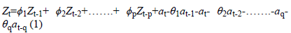
Here:  Parameter values for autoregressive operator; at:
Error term coefficients; θq: Parameter values for moving
average operator; Zt: Time series of the original series
differenced at degree d.
Parameter values for autoregressive operator; at:
Error term coefficients; θq: Parameter values for moving
average operator; Zt: Time series of the original series
differenced at degree d.
 (2)
(2)
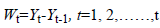
The first differences series is defined as given in the equation (2).
Wt=The first differences series,
Yt=The random variables subset of the original time series.
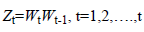
If the first differences series is not stationary, stationary is checked by differencing the first time series again. This is modeled as given in equation (3).
 (3)
(3)
When the degree of differencing is d=0 (that means that the original series is stationary), ARIMA model will be AR, MA, or ARMA model. Due to this feature, it can be said that ARIMA models incorporate all of the Box-Jenkins models [5].
Seasonal Box-Jenkins models are represented as ARIMA (p,q,d)(P,D,Q)s. Here, P is the degree of Seasonal Autoregressive (SAR) model; D is the number of seasonal differencing operations; Q is the order of Seasonal Moving Average (SMA) model; and s is the period. In a combined autoregressive moving average model, the future value of a variable is assumed to be a linear function of past observations and random errors [6]. Seasonal ARIMA (p,q,d) (P,D,Q)s models ARIMA (p,d,q) models relationship is represented in Equation (4). They are SARIMA models [7].
 at (4)
The model establishment process involves certain repetitive steps [3]. These steps are indicated in the flow chart given in Figure 1.

Figure 1: Model Establishment Process.
In determining the model, a model is selected from model classes such as AR, MA, ARMA, ARIMA, and SARIMA.
Then the parameters of the transient model are forecasted by use of efficient statistical techniques, and the standard errors of coefficients are calculated to test whether or not they are significant. In the last stage, compliance of the model is checked for forecasting. To this end, the autocorrelation function of the model is examined by drawing the graph of the autocorrelation coefficients of the errors of the transient model that is assumed to be compliant. If this function displays a particular shape, it is concluded that errors are not random. This kind of a finding means that the determined transient model is not compliant. Therefore, one turns to the second step again, and this process is repeated until the compliant model is determined through a new transient model. The model passing the compliance check is now ready to be used for forecasting [8].
Forecasting methods based on exponential smoothing and moving averages are also used in forecasting. Simple exponential smoothing method was derived from moving averages and is expressed as indicated in Equation (5) [9].
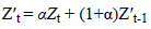 (5)
(5) 
Here,  refers to the forecast value for the forthcoming
period; α refers to smoothing coefficient (it takes a value in the
range of
refers to the forecast value for the forthcoming
period; α refers to smoothing coefficient (it takes a value in the
range of  refers to true index value in period t or
new observation; and
refers to true index value in period t or
new observation; and  refers to former smoothed value. The
most important point to consider at this point is the
determination of α so that mean square errors are minimized.
The seasonal ARIMA model or SARIMA model is an
expanded form of ARIMA, which allows for seasonal factors
to be reflected [10-13]. Holt’s two-parameter linear exponential
smoothing method equation is indicated in Equation (6) [14].
refers to former smoothed value. The
most important point to consider at this point is the
determination of α so that mean square errors are minimized.
The seasonal ARIMA model or SARIMA model is an
expanded form of ARIMA, which allows for seasonal factors
to be reflected [10-13]. Holt’s two-parameter linear exponential
smoothing method equation is indicated in Equation (6) [14].
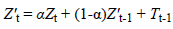

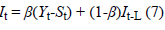
Here, 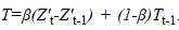 In addition, β and 1-β are the
parameters of the method and take a value between 0 and 1.
In addition, β and 1-β are the
parameters of the method and take a value between 0 and 1.
Brown’s exponential smoothing method is expressed as follows:
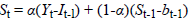
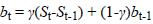
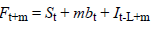
t is a value observed at time Yt; t is a seasonal component; bt is the smoothing component of the trend of t; L is the number of periods in a season; Ft+m is one forecast ahead of m periods; m is the number of forecasted periods; α is parameter smoothing; β is seasonal smoothing parameter; and γ is the smoothing parameter of the trend [15].
Goodness of fit criteria of the obtained models is evaluated through comparison with one another. R2 is a commonly known criterion. It is the goodness of fit criterion of the linear model. It is also known as coefficient of determination. It is in the range of 0-1 and smaller values indicate that the model does not have a good fit for the data. Stationary R2 is a criterion that compares the stationary part of the model and the basic model. It is preferred when there is a trend or seasonal pattern. RMSE is the square root of mean square errors. It is used for indicating how different dependent series are from the level forecasted by the model. Smaller values show that model forecasting is better. MAPE refers to mean absolute percentage error, is independent of the units of the series, and thus can be used in the comparison of different series. MAE refers to mean average error and is expressed with the series’ own units. MaxAPE is the maximum absolute percentage error measure. It indicates the highest error occurring among the forecasted values, is expressed in percentage, and thus unit independent. It is a measure that can be used for the worst scenarios among the forecasts. MaxAE is the maximum absolute error and is expressed in the same unit as the dependent series. Norm. BIC (Normalized Bayesyan Information Criterion) is the general measure of the total fit of the model. This measure is used for making a comparison between different models when the series are the same, and smaller values indicate a better model [16-18].
Results
MAPE values in the Tables 2 and 3 show that the best forecasting model is the Holt model among exponential smoothing and trend methods [19].
| Years | The Observed Number of Patients | Simple Exponential Smoothing | Holt Model | Brown Model | Linear Trend | Quadratic Trend | Exponential Trend | S curve |
|---|---|---|---|---|---|---|---|---|
| 2011 | 593 | 595 | 569.09 | 583.6 | -2374 | 1651.7 | 459 | 536.03 |
| 2012 | 583 | 598 | 548.04 | 572.62 | -2534 | 1778.6 | 440 | 518.31 |
| 2013 | 573 | 602 | 527.76 | 562.89 | -2695 | 1912.4 | 422 | 501.2 |
| 2014 | - | 605 | 508.24 | 554.54 | -2855 | 2052.9 | 405 | 484.68 |
| 2015 | - | 608 | 489.44 | 547.72 | -3016 | 2200.2 | 388 | 468.72 |
| 2016 | - | 612 | 471.33 | 542.55 | -3177 | 2354.2 | 373 | 453.31 |
| 2017 | - | 615 | 453.89 | 539.19 | -3337 | 2515 | 357 | 438.42 |
| 2018 | - | 619 | 437.1 | 537.79 | -3498 | 2682.6 | 343 | 424.04 |
| 2019 | - | 622 | 420.93 | 538.52 | -3658 | 2856.9 | 329 | 410.14 |
| 2020 | - | 626 | 405.36 | 541.59 | -3819 | 3038 | 315 | 396.72 |
Table 2: Exponential smoothing methods forecasts about the number of persons per physician between 2011 and 2020.
| Model | Simple Exponential Smoothing | Holt Model | Brown Model | Linear Trend | Quadratic Trend | Exponential Trend | S curve |
|---|---|---|---|---|---|---|---|
| MAPE | 6.332 | 5.252 | 5.716 | 89 | 31 | 14 | 12 |
Table 3: The comparison of exponential smoothing and trend models.
The Table 2, Table 3 and Figure 2 demonstrates that forecasting values based on the simple exponential smoothing method are appropriate for the period between 2010 and 2015, but reliability of forecasts falls for the period between 2016 and 2020.

Figure 2: The logarithm of the number of persons per physician by year and the Holt model forecasting graph of the values differenced at the first degree.
The Figure 3 presents a non-stationary display both in the variance and in the average. The Figure 4 takes the logarithm of the data but fails to achieve stationarity both in the variance and in the average. The Figure 5 differences at the first degree and takes the logarithm of the data and presents a stationary display both in the average and in the variance, though partly.

Figure 3: The pilot graph of the number of persons per physician by year.

Figure 4: The pilot graph of the values whose logarithm was taken for the number of persons.

Figure 5: The logarithm of the number of persons per physician by year and the pilot graph of the values differenced at the first degree.
In this instance, the autocorrelation (acf) graph (Figure 6) forecasts the coefficient of the MA model while the partial autocorrelation (pacf) graph (Figure 7) forecasts the coefficient of the AR model.

Figure 6: The autocorrelation (acf) graph of the values differenced at the first degree and the logarithm of the number of persons per physician by year.

Figure 7: The partial autocorrelation (pacf) graph of the values differenced at the first degree and the logarithm of the number of persons per physician by year.
Since the acf and pacf graphs of the models do not involve any diagram outside confidence limits, AR and MA models may be taken as 0.
The Table 4, Table 5 and Figure 8 indicates that the Box- Jenkins model method suggests that forecast values are appropriate for the years 2010 to 2016, but confidence interval gets some wider for the years 2017 to 2020, thereby leading to a fall in the reliability of forecasts.
| Model | Stationary R2 | R2 | RMSE | MAPE | MAE | MaxAPE | MaxAE | Norm.BIC |
|---|---|---|---|---|---|---|---|---|
| ARIMA (0,1,0) | -0.00044 | 0.986 | 512.436 | 5.395 | 248.814 | 105.224 | 3419.539 | 12.532 |
Table 4: ARIMA (0,1,0) Model fit statistics.
| Years | The number of observed patients | The number of persons per physician | Lower limit | Upper limit |
|---|---|---|---|---|
| 2011 | 593 | 572.5 | 466.6 | 695.2 |
| 2012 | 583 | 554.1 | 413.8 | 727.3 |
| 2013 | 573 | 536.4 | 374.1 | 746.3 |
| 2014 | - | 519.2 | 341.6 | 758.2 |
| 2015 | - | 502.6 | 313.9 | 765.5 |
| 2016 | - | 486.6 | 289.7 | 769.3 |
| 2017 | - | 471 | 268.3 | 770.6 |
| 2018 | - | 455.9 | 249.2 | 769.7 |
| 2019 | - | 441.3 | 232 | 767.2 |
| 2020 | - | 427.2 | 216.3 | 763.2 |
Table 5: Forecast values regarding the number of persons per physician by year for the Box-Jenkins model.

Figure 8: The Box-Jenkins model (ARIMA (0,1,0)) forecast graph of the values differenced at the first degree and the logarithm of the persons per physician by year.
The Table 6 illustrates, in summary, the goodness of fit criteria of the relevant models. It is seen that the ARIMA (0,1,0) model has the best values except for mean absolute percentage error The Figure 9 illustrates the graph of observed number of patients in three years and forecasts about the number of persons per physician in three years for the Holt model of the exponential smoothing method and the ARIMA (0,1,0) model of the Box-Jenkis method.
| Model | R2 | RMSE | MAPE | MAE | MaxAPE | MaxAE |
|---|---|---|---|---|---|---|
| HOLT MODEL | 0.986 | 515.088 | 5.252 | 245.017 | 105.934 | 3442.613 |
| ARIMA (0,1,0) | 0.986 | 512.436 | 5.395 | 248.814 | 105.224 | 3419.539 |
Table 6: The Goodness of fit criteria of the exponential smoothing and ARIMA (0,1,0) models.
The Figure 9 indicates that the forecasts by the ARIMA (0,1,0) model of the Box-Jenkis method are closer to the observed number of patients in comparison to the forecasts by the Holt model of the exponential smoothing method. However, since the difference is not too big, it can be said that the forecasts of both methods are good.

Figure 9: The Graph of the Holt Exponential Smoothing Model, the ARIMA (0,1,0) Model, and the Number of Observed Patients.
Discussion
This study aims to forecast the number of persons per physician in the future through predictive analysis by producing different models and determining the best models in this matter. Among the exponential smoothing models, the best predictive one was seen to be the Holt model. Among the Box Jenkins models, the best predictive one was seen to be the ARIMA (0,1,0) model.
The comparison of the above-mentioned best predictive models with one another was made based on the comparison of the forecast values of the models and the observed number of persons per physician in the first 3 years (2011, 2012, and 2013) and goodness of fit criteria. The Holt exponential smoothing model was found to be the best predictive model in terms of goodness of fit criteria in that it had a lower mean error in comparison to the other model. On the other hand, the ARIMA (0,1,0) model was seen to be the best predictive model in terms of the closeness of the forecasts regarding the first 3 years to the reality. The fact that the forecasts are quite close to the observed number of patients shows that these techniques can be used for forecasting the patient volume of hospitals and the sufficiency of staff. In this regard, more right and reliable policies may be developed for the health care industry through forecasts for the future.
According to the activity report data of the Ministry of Health for the year 2012, 124,219 physicians worked in Turkey at the end of 2012. Of these physicians, 68,262 were specialist physicians; 35,739 were practicing physicians; and 20,218 were physician assistants. The Health Transformation Programme has facilitated the access of the patients to the doctor. The number of cases of consulting a physician per person was 3.2 in 2002 but had risen to 8.3 by 2012. The total number of physicians in Turkey was 124,219 in 2012 when the number of physicians per one hundred thousand people was 165; that of practicing physicians was 48; that of specialist physicians was 90; that of dentists was 27; that of pharmacists was 34; and that of midwives and nurses was 232. Medical faculties have 45,732 registered students and 10,440 faculty members. The number of students per faculty member is 4.3. While the number of physicians per 1000 people is 3.3 in average in Europe, this figure is around 1.6 in Turkey. It implies a considerable physician shortage. On the other hand, the quotes of medical faculties in Turkey have been increasing rapidly. The total quote was 6492 in 2008, but went up to 8453 in 2012. Proper steps should be taken for a correct planning of the quantity and quality of physicians in Turkey.
Another important recommendation is that an independent institution should be responsible for the country-wide organization of the health information system. All public and private institutions, organizations, and people operating or working in the field of health should ensure data flow to this institution. Officials should be appointed and units should be set up to ensure such data flow in institutions and organizations of a size bigger than a specific size. Legislative regulations should be introduced to accelerate bureaucratic processes in this matter. All administrative works and functions such as planning, organization, management, and rearrangement of healthcare services should be based on the data/evidence to be provided by this institution. Likewise, the problems and effects of healthcare services should be evaluated based on the data of this institution.
References
- http://www.saglik.gov.tr/TR/dosya/1-82968/h/faaliyetraporu2012.pdf
- http://www.tuik.gov.tr/Kitap.do?KITAP_ID=158&KT_ID=0&metod=KitapDetay
- Box GEP, Jenkins GM. Time Series Analysis, Forecasting and Control, San Francisco: Holden-Day; 1976
- Işığıçok E. Causality Tests in Search of Relationships between Variables and an Application Testing. Doctoral Thesis. Uludağ University Institute of Social Sciences; 1993
- Box GEP, Jenkins GM, Reinsel GC. Time series analysis: Forecasting and control, 3rd ed. Englewood Cliffs, NJ: Prentice Hall; 1994.
- Brockwell PJ, Davis RA. Time Series: Theory and Methods, 2nd ed.: Springer-Verlag; 1991.
- Makridakis SG, Wheelwright SC, Hyndman RJ. Forecasting: Methods and applications, 3rd ed. New York: John Wiley and Sons; 1997.
- Yaman K, Sarucan A, Atak M, Aktürk N. Preparation of Data for Dynamic Scheduling Using Image Processıng and ARIMA Models. Gazi University J Faculty Eng Arch 2001; 16: 19-40.
- Box GBP, Jenkins GM, Reinsel GC, Liu LM. Time Series Analysis, 4th ed. Pearson Education; 2009.
- Kam HJ, Sung JO, Park RW. Prediction of Daily Patient Numbers for a Regional Emergency Medical Center using Time Series Analysis. Healthc Inform Res 2010; 16: 158-165.
- Moosazadeh M, Nasehi M, Bahrampour A, Khanjani N, Sharafi S, Ahmadi S. Forecasting Tuberculosis Incidence In Iran Using Box-Jenkins Models. Iran Red Crescent Med J 2014; 16: e11779.
- Soni K, Kapoor S, Parmar KS, Kaskaoutis DG. Statistical analysis of aerosols over the Gangetic–Himalayan region using ARIMA model based on long-term MODIS observations. Atmos Res 2014; 149: 174-219.
- Soni K, Parmar KS, Kapoor S. Time series model prediction and trend variability of aerosol optical depth over coal mines in India. Environ SciPollut Res 2015; 22: 3652-3671.
- Commandeur JJF, Koopman SJ. Introduction to State Space Time Series Analysis. Oxford University Press; 2007.
- Gardner ES, Exponential smoothing: The state of the art. J Forecasting 1985; 4: 1-28.
- Irmak S, Köksal CD, Asilkan Ö. Predicting Future Patient Volumes of the Hospitals by Using Data Mining Methods. Int J Alanya Faculty Business 2012; 4: 101-114.
- SPSS. Clementine11.1 User’s Guide, Integral Solutions Limited, Chicago, IL., 2007.
- SPSS. Clementine11.1 Node Reference, Integral Solutions Limited, Chicago, IL, 2007.
- Helfenstein U. Box-Jenkins modelling in medical research. Statistic Meth Med Res 1996; 5: 3.