ISSN: 0970-938X (Print) | 0976-1683 (Electronic)
Biomedical Research
An International Journal of Medical Sciences
Research Article - Biomedical Research (2018) Computational Life Sciences and Smarter Technological Advancement: Edition: II
Classification of alzheimer's disease subjects from MRI using fuzzy neural network with feature extraction using discrete wavelet transform
1Department of Computer Application, Sri Kanyakaparameswari Arts and Science College for Women, Chennai, India
2Department of Computer Science, Quaid –E-Millath Government College for Women, Chennai, India
- *Corresponding Author:
- Geetha C
Department of Computer Application
Sri Kanyakaparameswari Arts and Science College for Women, India
Accepted date: February 01, 2017
DOI: 10.4066/biomedicalresearch.29-16-2319
Visit for more related articles at Biomedical ResearchAlzheimer's Disease (AD) is a kind of dementia which is tricky to diagnose in accordance with clinical observations. Detection of Alzheimer’s diseases over brain Magnetic Resonance Imaging (MRI) data is main concern in the neurosciences. Traditional assessment of functional image scans typically relies on manual reorientation, visual reading and semi quantitative investigation of certain sections of the brain. Here, proposed Fuzzy Neural Network (FNN) scheme for the purpose of automated multiclass diagnosis of Dementia, in accordance with classification of MRI of human brain. During the initial stage of the work pre-processing is done to get rid of noises. The pre-processing and enhancement scheme includes two steps; initially the removal of film artifacts, for instance, labels and X-ray marks are eliminated from the MRI by means of tracking algorithm. Then, the elimination of high frequency elements by means of Ant Colony based Optimization (ACO) scheme. 2D histogram signal is obtained from preprocessed MR images of brain and subsequently further feature extraction is done through Discrete Wavelet Transform (DWT). This makes use of first few DWT coefficients as features and utilized for the purpose of classification by means of FNN. The features consequently derived are employed for the purpose of training a Fuzzy Neural Network (FNN) to classify features into three classes like Alzheimer’s, Mild Alzheimer's and Huntington's disease. The experimental result shows that the proposed method classification accuracy performance is better than other classification approaches.
Keywords
Preprocessing, Ant colony optimization, Fuzzy neural network, Discrete wavelet transform, 2D Histogram, X-ray marks
Introduction
Alzheimer's disease (AD) is the most common neurodegenerative dementia and a growing health problem. Definite diagnosis can only be made postmortem, and needs histopathological confirmation of amyloid plaques and neurofibrillary tangles. It considerably have an effect on one out of every 10 individuals above the age of 65” [1], and it “influences approximately 50-70% of people who is ill with from dementia” in a study by Diamond et al. [2]. This disease was named after the German psychiatrist and pathologist Alois Alzheimer after he inspected a female patient (post mortem) during 1906 that had died at age 51 following rigorous memory complications, confusion and also complicatedness in understanding questions. Alzheimer reported two common abnormalities in the brain of this patient, “1. Dense layers of protein deposited exterior and stuck between the nerve cells. 2. Regions of broken nerve fibers, within the nerve cells, which rather than being straight had become twisted”. Furthermore, these plaques and tangles have been employed in order to assist diagnosing of AD. “Amyloid plaques are sticky patches formed by insoluble proteins (Beta Amyloid) surrounded by the debris of dying nerve cells”. Amyloid plaques can be present with the normal aging process. “Neurofibrillary tangles result from alteration of a protein called tau, which helps support nerve cell structure”.
In AD, patients have a lot of plaques and tangles that are found. When there are high levels of beta amyloid there are generally reduced levels of acetylcholine. Acetylcholine is a neurotransmitter that a normal, healthy brain relies upon very heavily. When Acetylcholine levels fall too low in AD patients then memory and other brain functions become impaired. Even though it is known more regarding the brain now that when Alois Alzheimer existed, it is still don’t know the cause of dementia. According to the Alzheimer’s Association there are 3 phases of AD: preclinical, mild cognitive impairment due to AD, and dementia due to AD. Preclinical AD includes “Measureable transformations in biomarkers (for instance brain imaging and spinal fluid chemistry) that points out the extremely earliest indications of disease, prior to outward symptoms are noticeable” [3]. Mild cognitive impairment (MCI) due to AD also includes “mild changes in memory and thinking abilities that are evident-enough to be noticed and measured- but are not accompanied with injury that compromises day by day activities and execution”. Dementia due to AD involves “cognitive and behavioural symptoms that are exist and are of adequate severity to harm the patient’s ability to function in daily life”.
The symptoms of AD vary between patients, and it often depends on the phase of the disease that they are in. However there are some common symptoms in all AD patients such as, depression, delusions, hallucinations, and behavioral disturbances. These symptoms tend to progress as the disease progresses. The patient’s anxiety and frustrations build upon each other as they become more frustrated with themselves at not being able to remember normal everyday things. As the disease continues to progress the patient becomes more secluded from others because of their increasing uncertainty. After a while the patient becomes severely dependant on others. They will eventually die because their body becomes unable to fight infections or regulate normal functions. Even with all the symptoms and signs of AD, it can only be 100% diagnosed after the patient dies by examining the brain [2].
In this paper, Fuzzy Neural Network (FNN) method is proposed for the purpose of automated multiclass diagnosis of Dementia, in accordance with the classification of MRI of human brain. In the initial stage of the work pre-processing is done to remove noises. The pre-processing is used to remove the film artifacts such as labels and X-ray marks using tracking algorithm. Then high frequency components are removed using Ant Colony based Optimization (ACO) technique. 2D histogram signal is obtained from pre-processed MR images of brain and then further feature extraction is done by using Discrete Wavelet Transform (DWT). The proposed method uses first few DWT coefficients as features and used for classification using FNN. Consequently, the features derived are utilized for the purpose of training a Fuzzy Neural Network (FNN) to classify features into three classes such as Alzheimer’s, Mild Alzheimer's and Huntington's disease. The structure of the paper is organized as follows: The next Section 2 provides the related work. Section 3 presents the methodology of FNN. Experiments in Section 4 show the results of the proposed method, and make thorough investigation of each step. Section 5 concludes the paper, summarizes proposed contributions, and plans for future work.
Related Works
MRI classification task plays an important role in medical image retrieval, which is a part of decision making in medical image analysis. It involves grouping MRI scans into predefined classes or finding the class to which a subject belongs. There have been several attempts in the literature to automatically classify structural brain MRI as AD, MCI or NC. Among of the most common methods it is found that Voxel Based Morphometry (VBM) [4] which is an automatic tool. It allows an exploration of the differences in local concentration of gray matter and white matter. Tensor Based Morphometry (TBM) [5] was proposed to identify local structural changes from the gradients of deformations fields. Object Based Morphometry (OBM) [6] was introduced to perform shape analysis of anatomical structures and recently, features based morphometry (FBM) [7] was proposed as a method for relevant brain features comparison using a probabilistic model on local image features in scale-space. Some other studies focused on measuring morphological structure of a Region of Interest (ROI) known to be affected by AD such as the hippocampus region. In research investigations that analyze hippocampus atrophy, the following image analysis schemes are identified.
In study by Toews et al. [8], the author automatically segments the hippocampus and uses its volume for the classification. In addition to volumetric methods, several surface-based shape description approaches have been proposed to understand the development of AD. In a study by Chupin et al. [9], shape details in the structure of Spherical Harmonics (SH) have been utilized as features in the Support Vector Machine (SVM) classifier. In case of research by Genrardin et al. [10], Statistical Shape Models (SSMs) have been employed for the purpose of modelling the variability in the hippocampal shapes among the population. Hence, the image-based diagnostic of AD relies mainly on analysis of hippocampus. Nevertheless, the overall volumetric or shape investigation of the hippocampus does not illustrate the local transformation of its structure, which is helpful for diagnosis. ROI-based methods are time consuming and observer-dependent. Moreover, most of the approaches cited above were proposed for group analysis and cannot be used to classify individual patients. In order to overcome all these limitations, computer vision tools and visual image processing techniques have been developed to allow an automated detection of atrophy in the ROI.
Recently, Content Based Visual Information Indexing methods have been widely used for medical image analysis. But, few are the works that address the visual content of brain scans to extract information relative to AD. In case of research by Sakthivel et al. [11], the authors concentrated on incorporating several kinds of information, together with textual data, image visual characteristics extracted from scans in addition to direct user (doctor) input. In general, features can contain coefficients of a spectral transform of image signal, e.g. Fourier or Discrete Cosine Transform coefficients (DCT), statistics on image gradients etc. Features used to describe brain images are local binary patterns (LBP) and DCT.
In a study by Agrawal et al. [12] uses visual image similarity to help early diagnosis of Alzheimer. It proves the performance of user feedback for the purpose of brain image classification. In case of research by Rueda et al. [13], Circular Harmonic Functions and Scale Invariant Features Transform (SIFT) descriptors are computed around the hippocampus region. Then several modes of classification are used to compare images. In a study by Akgul et al. [14], the authors propose a ROI retrieval method for brain MRI, they use the LBP and Kanade-Lucas-Tomasi features to extract local structural information. In a study by Mizotin et al. [15], the authors use SIFT descriptors extracted from the whole subject’s brain for the purpose of classifying among brain with and without AD.
Some works [16] on MRI classification for AD diagnosis evaluate the suitability of the Bag-of-Visual-Words (BoVW) approach for automatic classification of MR images in the case of Alzheimer’s disease. It shows that the Bag-of-Features (BOF) scheme is capable of describing the visual details in order to discriminate healthy brains from those suffering from the AD. However, both works do not address the MCI case which has become an important construct in the study of AD. The BoVW model represents a whole brain scan or a ROI as a histogram of occurrence of quantized visual features, which are called visual words. The latter received the name of visual signature of an image/ROI.
The choice of the initial description space (features) is of a primary importance as it has to be adapted to the nature of the images. Indeed, despite the good performances of SIFT features reported in [16], there is still place for an intensive investigation of the descriptors choice. SIFT or their approximated version SURF [17], widely used in classification of general purpose image data sets, are not optimal for MRI with the lack of pronounced high frequency texture and clear structural models. Here, based on the work of Bay et al. [18], Circular Harmonic Functions (CHF) is taken and this gives interesting approximations of blurred and noisy signal [19].
Methods
In this section, the overview of proposed system and methodology are explained.
System overview
System overview illustrated in Figure 1. It shows that the working procedure of the proposed system. Initially the MRI data base is pre-processed using ACO. The preprocessing consists of two steps, first the removal of film artifacts such as labels and X-ray marks are removed from the MRI using tracking algorithm. Second, the removal of high frequency components using Ant Colony based Optimization (ACO) technique. Then the 2D histogram applied for pre-processed data. And then further feature extraction is done by using Discrete Wavelet Transform (DWT). The proposed method uses first few DWT coefficients as features and used for classification using FNN. Then FNN to classify features into three classes such as Alzheimer’s, Mild Alzheimer's and Huntington's disease.

Figure 1: Architecture of proposed system.
Pre-processing based on ant colony optimization
Pre-processing techniques is used to improve the detection of the suspicious region from Magnetic Resonance Image (MRI). The pre-processing and enhancement method consists of two steps; first the removal of film artifacts such as labels and Xray marks are removed from the MRI using tracking algorithm. Second, the removal of high frequency components used Ant Colony Optimization (ACO) technique. It gives high resolution MRI compare than median filter, Adaptive filter and spatial filter. The performance of the proposed method is also evaluated by means of peak single-to noise-ratio (PSNR), Average Signal-to-Noise Ratio (ASNR).
The first step of pre-processing using tracking functions involve those operations that are generally essential before the major data examination and extraction of details, and are commonly grouped as radiometric or geometric improvements. MRI includes film artifacts or label on it, for instance, patient name, age and marks. Film artifacts are eliminated by means of tracking algorithm. At this point, beginning from the primary row and initial column, the intensity value of the pixels is analyzed, consequently the threshold value of the film artifacts is found. It is to be noted that the threshold value is extremely more than that of the threshold value is eliminated from MRI. The high intensity value of film artifacts are eliminated from MRI. At some point in the elimination of film artifacts, the image includes salt and pepper noise.
Tracking algorithm for removal of film artifacts
Step 1: Examine the MRI and transform it in a two dimensional matrix.
Step 2: Choose the peak threshold value for the purpose of eliminating white labels.
Step 3: Keep flag value as 255.
Step 4: Choose pixels with intensity value is equal to 255.
Step 5: When the intensity value is 255 subsequently, the flag value is fixed to zero and as a result the labels are eliminated from MRI.
Step 6: If not skip to the subsequent pixel.
Then the removal of film artifacts MR brain images is preprocessed using Ant Colony Optimization (ACO) technique to remove the high frequency components of noise. In this proposed method, number of ants move on a 2-D image, stepping from one pixel to another to construct a pheromone matrix, which determine the noise high frequency information for each pixel location in the image to remove the noise of the image. The movement of the ants is directed by the local variation of the image’s intensity values. Image noise removal process has the following steps: first is the initialization process. After this pheromone matrix is constructed by the ACO when it further runs for N no. of iterations. Iterative process consists of construction process and update process. The last is decision process by which high frequency noise is determined.ACO optimizes the majority of complications through guide search of the solution space. ACO algorithm is completely based on fundamental activities of ants. While an ant moves through certain paths, it drops a substance called pheromone, which subsequently influences the selection of paths by the other ants. ACO metaheuristic engages solution construction through a graph. A lot of ants move through the solution space adding together solution constituents to partial solutions until they attain a comprehensive solution. The selection of the high frequency constituents completely depends on the pheromone substance of the paths and a heuristic assessment. MRI pixels are taken as nodes. During each stage of the construction, a particular ant k chooses the subsequent node by means of a probabilistic action selection rule, which states the probability with which ant k will decide to move from current node i to next node j:
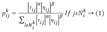
Where  indicates the pheromone substance of the arc from node i to node j,
  represents the neighborhood nodes for a specific ant k, provided that it is on node i. The neighborhood only comprises nodes that have not been visited by that specific ant k. When all possible nodes have been visited, after that the entire neighbors of the current node turn into available for visit. The constants α and ß indicates the influence of pheromone content and heuristic correspondingly. At last, ηij indicates the heuristic details for going from node i to node j. The heuristic information is a measure of the cost of extending the current partial solution. When a solution is formulated, it is assessed and the high frequency of pheromone is deposited proportionate to the quality of the solution. The ants deposit pheromone on the arcs they visited as given below:
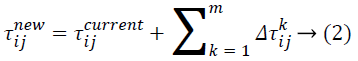
Where  indicates the quantity of pheromone ant k will put in to the arc travel from node i to node j, and m indicates the overall number of ants. The quantity of pheromone added is given as:
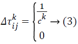
Ck indicates the overall cost of the path solution. The entire arcs in the equivalent path will have the similar cost value. Pheromone evaporation is also executed on all arcs following this equation:
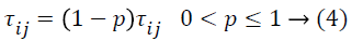
The last phermenon values are taken as the high frequency of noises. Subsequently, the noises are eliminated from the MRI.
2D Histogram signal representation
In this subsection, the pre-processed MRI are represented as 2D histogram signals. The histogram of an image indicates the relative frequency of amount of gray levels inside an image. Histogram-modeling schemes assist in modifying an image, in order that its histogram has a desired shape. This is helpful in stretching the low-contrast levels of an image with a narrow histogram, in that way realizing contrast enhancement. In case of Histogram Equalization (HE), the objective is to get hold of a consistent histogram for the output image, with the intention that an “optimal” overall contrast is perceived.
The Multidimensional histograms are the basically the extension of the concept of image histogram to multi-channel images. In case of image processing a 2D histogram, it illustrates the association of intensities during the exact place among the two images. The 2D histogram is typically employed for the purpose of comparing 2 channels in multichannel images, in which the x-axis indicate the intensities of the first channel and the y-axis the intensities of the second channel. At the same time as a comparison, a 1D histogram is nothing above counting the number of voxels with a specific intensity occurs in the image. The intensity limit of the image is partitioned in bins. A voxel subsequently belongs to the bin when its intensity is incorporated inside the range the bin represents. The 2D histogram is similar as the 1D histogram with the differentiation that it calculates the rate of combinations of intensities. The working out of a 2D histogram the images require to be identical in size.
Feature extraction from histogram MR image
The transformation of an image into its set of features is known as feature extraction. Useful features of the image are extracted from the image for classification purpose. It is a challenging task to extract good feature set for classification. In this paper, discrete wavelet transformation technique is used for feature extraction. The feature extraction process aims to take on the features of MRI Brain Images in the form of vector approximation at every level of wavelet decomposition. Feature extraction consists of four stages as follows: 1. Image decomposition using wavelet transformation. 2. Wavelet decomposition process is carried out. Wavelet types that will be used are Haar to level 3. The output coefficient vector is calculated using discrete wavelet transform.
By applying discrete wavelet transform, a number of sub-bands are generated. Initially, the continuous wavelet transform of a signal x(t), square-integrable function, and comparative to a real-valued wavelet, ψ(t) is given as [1]:
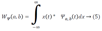
Where 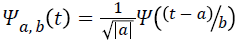 and the wavelet ψa,b is worked out from the mother wavelet ψ by means of translation and dilation process; a indicates the dilation factor and b represents the translation parameter. Based on few gentle assumptions, the mother wavelet ψ meets the constraint of having zero mean can be discretized by means of restraining a and b to a discrete lattice (a=2b, a ϵ R+, b ϵ R) to provide the DWT. At this point, the significant discrete wavelet of Haar wavelet is utilized. DWT is particularly a linear transformation and it functions on a data vector whose length is an integer power of two, converting it into a numerically different vector of the identical length. The wavelet coefficients are computed for the LL subband with the assistance of Haar wavelet
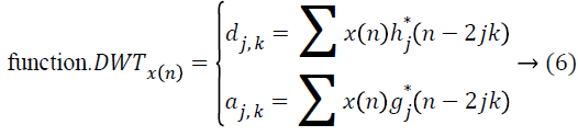
The coefficients dj,k refer to the detail components in signal x(n) and correspond to the wavelet function, while aj,k indicates the approximation components in the signal. The functions h(n) and g(n) indicates the coefficients of the highpass and low-pass filters, correspondingly, at the same time as parameters j and k indicates wavelet scale and translation factors. The major feature of DWT is multiscale representation of function. The histogram MRI is a process along the x and y direction through h(n) and g(n) filters which, is the row depiction of the original image. On account of this transform there are 4 sub-bands LL (lowlow), LH (low-high), HL (highlow), and HH (high-high) images at each scale. The sub-band image LL is used for DWT calculation at the next scale. The computation of wavelet features from histogram MRI is by means of spatial filtering and slice averaging, the wavelet coefficients are initially computed for the LL sub-band through Haar wavelet function.
Classification using fuzzy neural network
The extraction of feature sets is used for classification method. Fuzzy Neural Network (FNN) is used for MR brain image classification. The MR brain image classification result is based on three categories such as Alzheimer’s disease, Mild Alzheimer's disease and Huntington's disease. The performance of the classification method is also evaluated by accuracy, sensitivity and specificity.
FNN is executed in between the two classes. Every class grouping of the FNN works the similar manner. Additional classes yield fuzzy memberships in supplementary classes from which to choose a maximum value winner during the final output node. The features in the input are prototype feature vectors. At this point, there are two classes in the training exemplar data {x(q),t(q):q=1,…,Q}, i.e., the t(q) have two distinctive labels, as a result here utilized K=2 class groups of hidden nodes in which every such node indicates a Gaussian function centered on an exemplar feature vector that has a connected label. Every Gaussian in a class group has a dissimilar center however the same label. The initial group of hidden nodes are taken for Class 1. In the typical scenario, there might be a huge number Kр of feature vectors in Class р (here it is taken as p=1,2), as a result those feature vectors that are near to a different feature vector with the identical label is eradicated. This considerably lessens the amount of centers, and as a result Gaussians (nodes), that indicate each Class p. The fuzzy truth that input vector is in the similar class as x(q) is given through the Gaussian Fuzzy Set Membership Function (FSMF) centered on x(q). The Gaussian FSMF is the function which is given as,
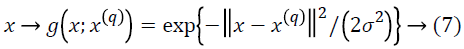
Where σ is considered as one-half of the average distance among the entire exemplar pairs.
At this moment, the entire fuzzy facts for the centers of Gaussians in Class 1 are fed from their Gaussian nodes to the maximizer node of the Class 1 fuzzy truths, which performs as a fuzzy OR node in choosing the representative center and fuzzy truth that x belongs to certain x(k) for Class 1. This maximum fuzzy truth for x in Class 1 is now given to the final output maximizer node as the Class 1 representative. In addition, the last output maximizer node receives the Class 2 representative (maximum fuzzy truth) that belongs to Class 2 and concludes the maximum of these fuzzy truths, as a result the class that sent it is the winner. Accordingly, the input belongs to the winning class decided with the label of the winning Gaussian center vector.
Algorithm for fuzzy neural network classification
The high level algorithm is almost clear-cut as provided in the steps given below, and is uncomplicated to proceed with the program. The training and learning reside in the exemplar feature vector and their labels don’t require expending computation time for the purpose of training. The pseudo code algorithm is given as follows.
Step 1: Get the data file (the amount of features N, the quantity of feature vectors Q, the dimension J of the labels, the number K of classes, the entire Q feature vectors and the entire Q labels).
Step 2: Discover minimal distance Dmin over the entire feature vector pairs
Put σ =Dmin/2
Put G=Q//starting no. of Gaussian centers
Step 3: Discover two exemplar vectors of min. distance with indices k1 and k2.
If d<(1/2) Dmin // if vector are close
If label[k1] = label[k2]//have same lable
Eliminate Gaussian k2
G=G-1//reduce no. of Gaussians
Go to step 2
Step 4: Input next unknown x to SFNN to be classified
For k=1 to G do
Compute g[k]=exp{-||x-x(k)||2/(2σ2)}
Find maximum g[k*], ober k=1,…,G
Output x, label [k*]//label [k*] is class of x
Step 5: If all inputs for classifying are done, stop Else, go to Step 3.
Results
In this section, performance of proposed DWT with FNN classifier is evaluated. The experiments were carried out on the matlab platform. The datasets includes T2-weighted MRI in axial plane and 256 × 256 in-plane resolution, which were obtained from the website of Harvard Medical School (URL: http://med.harvard.edu/AANLIB/), OASIS dataset (URL: http://www.oasis-brains.org/), and ADNI dataset (URL: http://adni.loni.uc-la.edu/). After that choose T2 model since T2 images are of higher-contrast and better vision when compared against the T1 and PET modalities. The abnormal brain MRI of the dataset consists of the following diseases: Alzheimer's disease, Alzheimer's disease plus visual agnosia. The samples of every disease are shown in Figure 2. A total of 20 images were randomly chosen for every category of brain. Since there are one category of normal brain and seven categories of abnormal brain in the dataset, 160 images are chosen consisting of 20 normal and 140 (=7 categories of diseases 20 images/diseases) abnormal brain images.

Figure 2: a) Normal brain MR images; b) Alzheimer’s disease; c) Alzheimer’s disease plus visual agnosia.
The proposed DWT with FNN classifier is compared with the existing Discrete Cosine Transform (DCT) with Artificial Neural Network (ANN) and Support Vector Machine (SVM) classifier. In the classification result is based on four classes such as Alzheimer’s disease, Mild Alzheimer's disease, Huntington's disease and normal. In the classification problem, it is identified as positives the class and as negatives the class. Doing so, the following standard definitions are obtained: 1) True Positives (TP): predicts class as class. 2) True Negatives (TN): predicts non-class as class. 3) False Positives (FP): predicts non-class as non-class. 4) False Negatives (FN): predicts class as non-class. As a consequence, the following standard definitions are obtained:
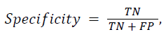
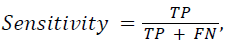
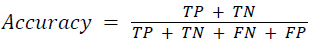
Some preliminary results, in terms of sensitivity, specificity, and accuracy are reported in Table 1 for the MR brain images.
| Classification Methods | Accuracy (%) | Specificity (%) | Sensitivity (%) |
|---|---|---|---|
| DWT With FNN classifier | 95.5 | 86 | 88 |
| DCT with ANN classifier | 92.8 | 80 | 82 |
| SVM classifier | 89.8 | 76 | 80 |
Table 1: Overall comparison results.
Peak signal to noise ratio (PSNR)
It is the ratio between the utmost possible powers to the power of corrupting noise is given as Peak Signal to Noise Ratio. It considerably has an effect on the fidelity of its representation. It can be also observed that it is the logarithmic function of peak value of image and Mean Square Error (MSE).
PSNR = 10 log10(MAX2i/MSE)
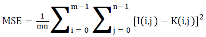
Mean square error
Mean Square Error (MSE) of an estimator is to quantify the difference between an estimator and the true value of the quantity being estimated.
Accuracy comparison
The proposed DWT with FNN classifier produces better accuracy rate shown in Figure 3 which is much greater accuracy results than existing DCT with ANN classifier and SVM classifier. When the number of images increases the accuracy of the result is increases. This approach produces high accuracy rate when compared to existing system.

Figure 3: Accuracy vs. No of images.
Sensitivity comparison
The proposed DWT with FNN classifier produces high sensitivity shown in Figure 4 which is much greater accuracy results than existing DCT with ANN classifier and SVM classifier. When the number of images increases the sensitivity of the result is increases. This approach produces high sensitivity rate when compared to existing system.

Figure 4: Sensitivity vs. no of images.
Specificity comparison
The proposed DWT with FNN classifier produces high specificity shown in Figure 5 is higher than the existing DCT with ANN classifier and SVM classifier. When the number of features increases the specificity of the result is increases. This approach produces effective specificity rate when compared to existing system.

Figure 5: Specificity vs. no of images.
Peak signal to noise ratio (PSNR)
To measure the perceptual quality, after the attacks are added to MR brain images, then calculate the peak of signal-to-noise ratio (PSNR) that is used to estimate the quality of the preprocessing MR brain images in comparison with the original ones. The performance of the proposed DWT with FNN classifier is compared with the existing DCT with ANN classifier and SVM classifier. The PSNR results of the proposed DWT with FNN classifier is higher when compare to existing DCT with ANN classifier and SVM classifier is shown in Figure 6.

Figure 6: Experimental results of PSNR comparison.
Mean square error
The performance of the DWT with FNN classifier is compared with the existing watermarking DCT with ANN classifier and SVM classifiers for MSE comparison. In the proposed work DWT with FNN classifier is measured between the MR brain images, it shows that the MSE results of the proposed DWT with FNN classifier have less MSE error rate is shown in Figure 7.

Figure 7: Experimental results of MSE comparison.
Conclusion
In this paper a simple and robust classification approach of MRI scans is proposed for Alzheimer’s disease diagnosis. The proposed FNN method is used for automated multiclass diagnosis of Dementia and the classification based on of human brain MR images. In the initial stage of the work preprocessing is done to remove noises. Then Ant Colony based Optimization ACO technique used for remove the high frequency components. 2D histogram signal is obtained from pre-processed MR images of brain and then further feature extraction is done by using DWT. The features hence derived are utilized for the purpose of training a FNN in order to classify the features into three classes like Alzheimer’s, Mild Alzheimer's and Huntington's disease. Also the experimental result demonstrated that the proposed method provides better classification accuracy compared to other volumetric methods. In the perspective of this work, it is planned to use other classification methods, however also multiple MRI modalities in the established classification framework.
References
- Colombo M, Kuo G, Choo QL, Donato MF, Del Ninno E, Tommasini MA, Dioguardi N, Houghton M. Prevalence of antibodies to hepatitis C virus in Italian patients with hepatocellular carcinoma. Lancet 1989; 2: 1006-1008.
- Diamond E, Miller S, Rentz D, Sperling R, Dickerson B, Atri A, Sperling RA. Relationship of fMRI activation to clinical trial memory measures in Alzheimer disease. Neurology 2007; 69: 1331-1341.
- Pah-Lavan Z. Alzheimer's disease: the road to oblivion. J Commun Nursing 2006; 20: 4-10.
- Pies RW. Alzheimer's Redux: A preliminary take on the new diagnostic criteria. Psychiatric Times 2012; 4: 24-30.
- Ashburner J, Friston KJ. Voxel-Based Morphometry-the methods. Neuroimage 2000; 11: 805-821.
- Wolz R, Julkunen V, Koikkalainen J, Niskanen E, Zhang DP, Rueckert D, Soininen H, Lötjönen J; Alzheimer's Disease Neuroimaging Initiative. Multi-method analysis of MRI images in early diagnostics of Alzheimer's disease. PLoS One 2011; 6: e25446.
- Mangin JF, Rivière D, Cachia A, Papadopoulos-Orfanos D, Collins DL, Evans AC, Régis J. Object-based strategy for morphometry of the cerebral cortex. Inf Process Med Imaging 2003; 18: 160-171.
- Toews M, Wells W, Collins DL, Arbel T. Feature-Based Morphometry: Discovering Group-related Anatomical Patterns. Neuro Image 2010; 49: 2318-2327.
- Chupin M, G´erardin E, Cuingnet R. Fully automatic hippocampus segmentation and classification in Alzheimer’s disease and mild cognitive impairment applied on data from ADNI. Hippocampus 2009; 19: 579-587.
- Gerardin E, Ch´etelat G, Chupin M. Multidimensional classification of hippocampal shape features discriminates Alzheimer’s disease and mild cognitive impairment from normal aging. Neuro Image 2009; 47: 1476-1486.
- Sakthivel K, Jayanthiladevi A, Kavitha C. Automatic detection of lung cancer nodules by employing intelligent fuzzy cmeans and support vector machine. Biomed Res 2016; 27: S123-S127.
- Agarwal M, Mostafa J. Image retrieval for Alzheimer disease detection. In: Proceedings of the First MICCAI international conference on Medical Content-Based Retrieval for Clinical Decision Support, Springer-Verlag, Berlin, Heidelberg, MCBR-CDS’09, 2010.
- Rueda A, Arevalo JE, Cruz-Roa A, Romero E, Gonz´alez FA. Bag of features for automatic classification of Alzheimer’s disease in Magnetic Resonance Images. In: CIARP, 2012.
- Akg¨ul CB, Unay D, Ekin A. Automated diagnosis of Alzheimer’s disease using image similarity and user feedback. In: Proceedings of the ACM International Conference on Image and Video Retrieval, ACM, New York, NY, USA, CIVR ’09, 2009.
- Mizotin M, Benois-Pineau J, Allard M, Catheline G. Feature-based brain MRI retrieval for Alzheimer disease diagnosis. In: 19th IEEE International Conference on Image Processing (ICIP), 2012.
- Ahmed OB, Jenny BP, Allard M, Amar CB, Catheline G. Classification of Alzheimer’s disease subjects from MRI using hippocampal visual features. Multimedia Tools and Applications, Springer, Verlag, 2014.
- Daliri MR. Automated Diagnosis of Alzheimer disease using the ScaleInvariant Feature Transforms in Magnetic Resonance Images. J Med Syst 2012; 36: 995-1000.
- Bay H, Ess A, Tuytelaars T, Van Gool L. Speeded-Up Robust Features (SURF). Comput Vis Image Underst 2008; 110: 346-359.
- Ben Ahmed O, Benois-Pineau J, Ben Amar C, Allard M, Catheline G. Early Alzheimer disease detection with bag-of-visual-words and hybrid fusion on structural MRI. In: 11th International Workshop on Content-Based Multimedia Indexing (CBMI) 2013, IEEE, 2013.